6.9. zeus: Sampling from multimodal distributions¶

Copied from the zeus documentation at https://zeus-mcmc.readthedocs.io/en/latest/index.html.

In this recipe we will demonstrate how one can use zeus with the Moves interface to sample efficiently from challenging high-dimensional multimodal distributions.

We will start by defining the target distribution, a 50-dimensional mixture of Normal distributions with huge valleys of almost-zero probability between the modes. This is an extremelly difficult target to sample from and most methods would fail.

import zeus 

import numpy as np
import matplotlib.pyplot as plt
import seaborn as sns 

# Number of dimensions
ndim = 50

# Means
mu1 = np.ones(ndim) * (1.0 / 2)
mu2 = -mu1

# Standard Deviations
stdev = 0.1
sigma = np.power(stdev, 2) * np.eye(ndim)
isigma = np.linalg.inv(sigma)
dsigma = np.linalg.det(sigma)

w1 = 0.33  # one mode with 0.1 of the mass
w2 = 1 - w1 # the other mode with 0.9 of the mass

# Uniform prior limits
low = -2.0
high = 2.0

# The log-likelihood function of the Gaussian Mixture
def two_gaussians(x):
    log_like1 = (
        -0.5 * ndim * np.log(2 * np.pi)
        - 0.5 * np.log(dsigma)
        - 0.5 * (x - mu1).T.dot(isigma).dot(x - mu1)
    )
    log_like2 = (
        -0.5 * ndim * np.log(2 * np.pi)
        - 0.5 * np.log(dsigma)
        - 0.5 * (x - mu2).T.dot(isigma).dot(x - mu2)
    )
    return np.logaddexp.reduce([np.log(w1) + log_like1, np.log(w2) + log_like2])

# A simple uniform log-prior
def log_prior(x):
    if np.all(x>low) and np.all(x<high):
        return 0.0
    else:
        return -np.inf

# The Log-Posterior
def log_post(x):
    lp = log_prior(x)
    if not np.isfinite(lp):
        return -np.inf
    return lp + two_gaussians(x)

A failed attempt¶

Now lets run zeus for 1000 steps using 100 walkers and see what happens:

nwalkers = 400
nsteps= 2000

# The starting positions of the walkers
start = low + np.random.rand(nwalkers,ndim) * (high - low)

# Initialise the Ensemble Sampler
sampler = zeus.EnsembleSampler(nwalkers, ndim, log_post)
# Run MCMC
sampler.run_mcmc(start, nsteps)

# Get the samples
samples = sampler.get_chain()

# Plot the walker trajectories for the first parameter of the 10
plt.figure(figsize=(16,4))
plt.plot(samples[:,:,0],alpha=0.5)
plt.show()

Initialising ensemble of 400 walkers...
Sampling progress : 100%|█████████| 2000/2000 [03:53<00:00,  8.55it/s]

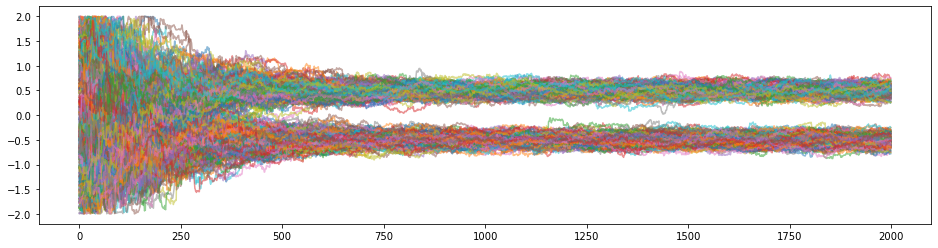
As you can see, once the walkers have found the modes/peaks of the Gaussian Mixture they stay stranded there, unable to jump to the other modes. This is a huge issue because it prevents the walkers from distributing the probability mass fairly among the peaks thus leading to biased results.

The clever way…¶

Now that we know that our target is multimodal, and that the default DifferentialMove cannot facilitate jumps between modes we can use a more advanced move such as the GlobalMove.

Although the GlobalMove is a very powerful tools, it is not well suited during the burnin phase. For that reason we will use the default DifferentialMove during burnin and then bring out the big guns.

# Initialise the Ensemble Sampler using the default ``DifferentialMove``
sampler = zeus.EnsembleSampler(nwalkers, ndim, log_post)
# Run MCMC
sampler.run_mcmc(start, nsteps)

# Get the burnin samples
burnin = sampler.get_chain()

# Set the new starting positions of walkers based on their last positions
start = burnin[-1]

# Initialise the Ensemble Sampler using the advanced ``GlobalMove``.
sampler = zeus.EnsembleSampler(nwalkers, ndim, log_post, moves=zeus.moves.GlobalMove())
# Run MCMC
sampler.run_mcmc(start, nsteps)

# Get the samples and combine them with the burnin phase for plotting purposes
samples = sampler.get_chain()
total_samples = np.concatenate((burnin, samples))

# Plot the walker trajectories for the first parameter of the 10
plt.figure(figsize=(16,4))
plt.plot(total_samples[:,:,0],alpha=0.5)
plt.show()

Initialising ensemble of 400 walkers...
Sampling progress : 100%|█████████| 2000/2000 [03:44<00:00,  8.90it/s]
Initialising ensemble of 400 walkers...
Sampling progress : 100%|█████████| 2000/2000 [09:24<00:00,  3.54it/s]

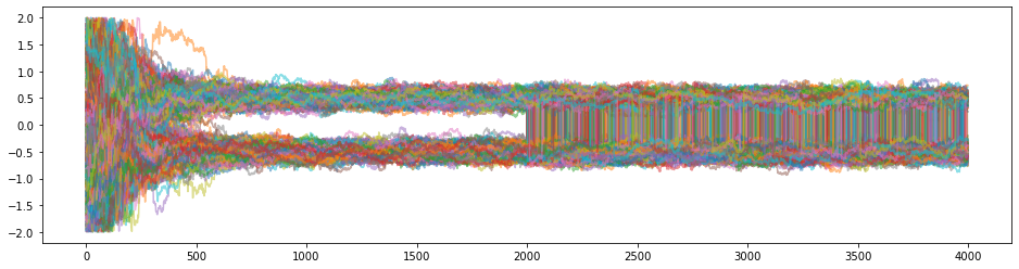
You can see that the moment we switched to the GlobalMove the walkers begun to jump from mode to mode frequently.

Lets now plot the 1D distribution of the first parameter and compare this with “actual truth”.

# Compute true samples from the gaussian mixture directly
s1 = np.random.multivariate_normal(mu1, sigma,size=int(w1*200000))
s2 = np.random.multivariate_normal(mu2, sigma,size=int(w2*200000))
samples_true = np.vstack((s1,s2))

# Get the chain from zeus
chain = sampler.get_chain(flat=True, discard=0.5)

# Plot Comparison
plt.figure(figsize=(8,6))
sns.kdeplot(chain[:,0])
sns.kdeplot(samples_true[:,0], ls='--')
plt.legend(['zeus - Global Move', 'Truth']);

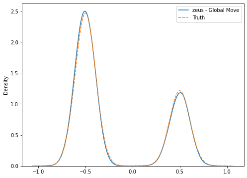
Using the advanced moves, the walkers can move great distances in parameter space.

Learning from data

6.9. zeus: Sampling from multimodal distributions¶

A failed attempt¶

The clever way…¶