2.1. Lecture 4: Parameter estimation¶

Overview comments¶

In general terms, “parameter estimation” in physics means obtaining values for parameters (i.e., constants) that appear in a theoretical model that describes data. (Exceptions exist, of course.)
Examples:
- couplings in a Hamiltonian
- coefficients of a polynomial or exponential model of data
- parameters describing a peak in a measured spectrum, such as the peak height and width (e.g., fitting a Lorentzian line shape) and the size of the background
- cosmological parameters such as the Hubble constant
Conventionally this process is known as “fitting the parameters” and the goal is to find the “best fit” and maybe error bars.
We will make particular interpretations of these phrases from our Bayesian point of view.
Plan: set up the problem and look at how familiar ideas like “least-squares fitting” show up from a Bayesian perspective.
As we proceed, we’ll make the case that for physics a Bayesian approach is particular well suited.

What can go wrong in a fit?¶

As a teaser, let’s ask: what can go wrong in a fit?

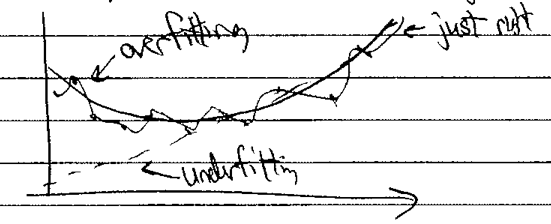
Bayesian methods can identify and prevent both underfitting (model is not complex enough to describe the fit data) or overfitting (model tunes to data fluctuations or terms are underdetermined, leading to them playing off each other).
$\Longrightarrow$ we’ll see how this plays out.

Notebook: Gaussian noise¶

Let’s step through Parameter estimation example: Gaussian noise and averages.

Import of modules
- Using seaborn just to make nice graphs
- We’ll use emcee here (cf. “MC” $\rightarrow$ “Monte Carlo”) to do the sampling.
- corner is used to make a particular type of plot.
Example from Sivia’s book [SS06]: Gaussian noise and averages.

\[ p(x | \mu,\sigma) = \frac{1}{\sqrt{2\pi\sigma^2}} e^{-\frac{(x-\mu)^2}{2\sigma^2}} \]

where $\mu$ and $\sigma$ are given and the pdf is normalized ($\int_{-\infty}^{+\infty} \frac{1}{\sqrt{2\pi}\sigma}e^{-(x-\mu)^2/2\sigma^2} dx = 1$).

Question

What are the dimensions of this pdf?

Answer

one over length ($1/x$) or one over what units $x$ is in.

Its justification as a theoretical model is via maximum entropy, the “central limit theorem” (CLT), or general considerations, all of which we will come back to in the future.
$M$ data measurements $D \equiv \{x_k\} = (x_1, \ldots, x_M)$ (e.g., $M=100$), distributed according to $p(x|\mu,\sigma)$ (that implies that if you histogrammed the samples, they would roughly look like the Gaussian).
How do we get such measurements? As in the Exploring PDFs notebook, we “sample” from $\mathcal{N}(\mu,\sigma^2)$.
Goal: given the measurements $D$, find the approximate $\mu$ and $\sigma$.
- Frequentist: use the maximum likelihood method
- Bayesian: compute posterior pdf $p(\mu,\sigma|D,I)$
Random seed of 1 means the same series of “random” numbers are used every time you repeat. If you put 2 or 42, then a different series from 1 will be used, but still the same with every run that has that seed.
stats.norm.rvs (“norm” for normal or Gaussian distribution; “rvs” for random variates) as in Exploring PDFs.
- size=M is a “keyword argument” (often kw $\equiv$ keyword), which means it is optional and there is a default value (here the default is $M=1$).
shift-tab-tab after evaluating a cell will give you information
- e.g., put your cursor on “norm” or “rvs” and shift-tab-tab will tell you all about these.
The output $D$ is a numpy array. (Everything in Python is an object, so more than just a datatype, there are methods that go with these arrays.)
- Put your cursor just after D and shift-tab-tab
- $[\cdots]$ when printed.
Consider the number of entries in the tails, say beyond $2\sigma$ $\Longrightarrow$ $x>12$ or $x < 8$.
- How many do you expect on average? $2\sigma$ means about 95%, so about 5/100.
- Here there are 4 in that range. If there were zero is there a bug? No, there is a chance that will happen!
Note the pattern (or lack of pattern) and repeat to get different numbers. (How? Change the random seed from 1.) Always play!
Questions about plotting? Some notes:
- We’ll repeatedly use constructions like this, so get used to it!
- ; means we put multiple statements on the same line; this is not necessary and probably should be avoided in most cases.
- alpha=0.5 makes the (default) color lighter.
- Try color='red' on your own in the scatter plot.
- You might prefer side-by-side graphs $\Longrightarrow$ alternative code.
- An “axis” in Matplotlib means an entire subfigure, not just the x-axis or y-axis.
- If you want to know about a potting command already there, shift-tab-tab (or you can always google it).
- To find vlines (vertical lines), google “matplotlib vertical line”. (Try it to find horizontal lines.)
- fig.tight_layout() for good spacing with subplots.
Observations on graphs?
- Scatter plot shows tail $\Longrightarrow$ in this case there are 5, but rerun and it will be more or less $\Longrightarrow$ everything is a pdf.
- The histogram is imperfect. Is this a problem? cf. the end of Exploring PDFs with different numbers of samples.
- Tails fluctuate!
Frequentist approach
- true value for parameters $\mu,\sigma$, not a pdf
- Use of $\mathcal{L}$ is common notation for likelihood.
- Why the product? Assumed independent. Reasonable?
- $\log\mathcal{L}$ for several reasons.
  - to avoid problems with extreme values
  - note: “$\log$” always means $\ln$. If we want base 10 we’ll use $\log_{10}$.
  - $\mathcal{L} = (\text{const.})e^{-\chi^2}$ so maximizing $\mathcal{L}$ is same as maximizing $\log\mathcal{L}$ or minimizing $\chi^2$.
Carry out the maximization

\[ \frac{\partial\log\mathcal{L}}{\partial\mu} = -\frac{1}{2}\sum_{i=1}^M 2 \frac{x_i-\mu}{\sigma^2}\cdot (-1) = \frac{1}{\sigma^2}\sum_{i=1}^M (x_i-\mu) = \frac{1}{\sigma^2}\Bigl(\bigl(\sum_{i=1}^M x_i\bigr) - M\mu\Bigr) \]

Set equal to zero to find $\mu_0$ $\Longrightarrow$ $M\mu_0 = \sum_{i=1}^M x_i$ or $\mu_0 = \frac{1}{M}\sum_{i=1}^M x_i$.

You do $\sigma_0^2$! (Easier to do $d/d\sigma^2$ than $d/d\sigma$.)
- Do these make sense?
  - $\mu_0$ is the mean of data $\rightarrow$ estimator for “true mean”.
  - $\sigma_0$ gives spread about $\mu_0$.
- Note the use of .sum to add up the $D$ array elements.
- Printing with f strings: f'...'
  - .2f means a float with 2 decimal places.
- Note comment on “unbiased estimator”
  - an accurate statistic
  - Here compare $\mu_0$ estimated from $\frac{1}{M}$ vs. $\frac{1}{M-1}$.
  - If you do this many times, you’ll find that $\frac{1}{M}$ doesn’t quite give $\mu_{\rm true}$ correctly (take mean of $\mu_0$s from many trials) but $\frac{1}{M-1}$ does!
  - The difference is $\mathcal{O}(1/M)$, so small for large $M$.
- Compare estimates to true. Are they good estimates? How can you tell? E.g., should they be within 0.1, 0.01, or what? (More about this as we proceed!)
Bayesian approach $\Longrightarrow$ $p(\mu,\sigma|D,I)$ is the posterior: the probability (density) of finding some $\mu,\sigma$ given data $D$ and what else we know ($I$).
- $I$ could be that $\sigma > 0$ or $\mu$ should be near zero.

Frequentist probability

Long-run frequency of (real or imagined) trials $\Longrightarrow$ data is probabilistic (repeat experiment and get different result) but model parameters are not (universe stays the same with more observations).

Bayesian probability

Quantification of information (what you know, often said as “what you believe”). Data are fixed (it’s what you found) but knowledge of true model parameters is fuzzy (and gets updated with more trials, cf. coin flipping).

One more time with Bayes’ theorem:

(2.1)¶\[ p(\mu,\sigma | D,I) = \frac{p(D | \mu,\sigma,I)\,p(\mu,\sigma|I)}{p(D|I)} \]

Label each term in Eq. (2.1).

\[ \underbrace{p(\mu,\sigma | D,I)}_{\text{posterior}} = \frac{\overbrace{p(D | \mu,\sigma,I)}^{\text{likelihood}}\ \ \overbrace{p(\mu,\sigma|I)}^{\text{prior}}}{\underbrace{p(D|I)}_{\text{evidence or data probability}}} \]

Bayes’ Theorem tells you how to flip $p(\mu,\sigma|D,I) \leftrightarrow p(D|\mu,\sigma,I)$. Here the first pdf is hard to think but evaluating but the second pdf is easy.

Note

Aside on the denominator, which is called in various contexts the evidence, the data probability, or the fully marginalized likelihood. We evaluate it by using the basic marginalization rule (from the sum rule) to first insert an integration over all values of the general vector of parameters $\boldsymbol{\theta}$ and then the product rule to obtain an integral over the probability to get the data $D$ given a particular $\boldsymbol{\theta}$ times the probability of that $\boldsymbol{\theta}$:

\[\begin{split} \begin{align} p(D|I) &= \int p(D,\boldsymbol{\theta}| I) \, d\boldsymbol{\theta} \\ &= \int p(D|\boldsymbol{\theta}, I) p(\boldsymbol{\theta})\, d\boldsymbol{\theta} \end{align} \end{split}\]

This is numerically a costly integral. Later we will look at ways to evaluate it.

For model fitting (i.e., parameter estimation), we don’t need $p(D|I)$ calculated. Instead we find the posterior and directly normalize that function or, most often we only need relative probabilities.
If $p(\mu,\sigma | I) \propto 1$, this is called a “flat” or “uniform” prior, in which case

\[ p(\mu,\sigma | D,I) \propto \mathcal{L}(D|\mu,\sigma) \]

and a Frequentist and Bayesian will get the same answer for the most likely values $\mu_0,\sigma_0$ (called “point estimates” as opposed to a full pdf).

We will argue against the use of uniform priors later.
The prior includes additional knowledge (information). It is what you know before the measurement in question.

Discussion point

A frequentist claims that the use of a prior is nonsense because it is subjective and tied to an individual. What would a Bayesian statistician say?

To compute posteriors such as $p(\mu,\sigma|D,I)$ in practice we often use Markov Chain Monte Carlo aka MCMC. We’ll look at it now and discuss later.

Notebook: Fitting a line¶

Look at Parameter estimation example: fitting a straight line.

Annotations of the notebook:

same imports as before
assume we create data $y_{\rm exp}$ (“exp” for “experiment”) from an underlying model of the form

\[ y_{\rm exp}(x) = m_{\rm true} x + b_{\rm true} + \mbox{Gaussian noise} \]

where

\[ \boldsymbol{\theta}_{\rm true} = [b_{\rm true}, m_{\rm true}] = [\text{intercept, slope}]_{\rm true} \]
The Gaussian noise is taken to have mean $\mu=0$ and standard deviation $\sigma = dy$ independent of $x$. This is implemented as y += dy * rand.randn(N) (note randn).
The $x_i$ points themselves are also chosen randomly according to a uniform distribution $\Longrightarrow$ rand.rand(N).
Here we are using the numpy random number generators while we will mostly use those from scipy.stats elsewhere.

The theoretical model $y_{\rm th}$ is:

\[ y_{\rm th} = m x + b, \quad \mbox{with}\ \theta = [b, m] \]

So in the sense of distributions (i.e., not an algebraic equation),

\[ y_{\rm exp} = y_{\rm th} + \delta y_{\rm exp} + \delta y_{\rm th} \]

The last term, which is the model discrepancy (or “theory error”) will be critically important in many applications, but has often been neglected. More on this later!
Here we’ll take $\delta y_{\rm th}$ to be negligible, which means that

\[ y_i \sim \mathcal{N}(y_{\rm th}(x_i;\boldsymbol{\theta}), dy^2) \]
- The notation here means that the random variable $y_i$ is drawn from a normal (i.e., Gaussian) distribution with mean $y_{\rm th}(x_i;\boldsymbol{\theta})$ (first entry) and variance $dy^2$ (second entry).
- For a long list of other probability distributions, see Appendix A of BDA3, which is what everyone calls Ref. [GCS+13].
We are assuming independence here. Is that a reasonable assumption?

Why Gaussians tend to show up¶

We’ll have several reason to explain why Gaussian distributions seem to show up everywhere. Here is a general reason. Given $p(x | D,I), then if the shape is not multimodal (only one hump), we could argue that our “best estimate” is

\[ \left.\frac{dp}{dx}\right|_{x_0} = 0 \quad \mbox{with} \quad \left.\frac{d^2p}{dx^2}\right|_{x_0} < 0 \ \text{(maximum)}. \]

To characterize the posterior $p(x)$, we look nearby. $p(x)$ itself varies too fast, but since it is positive definite we can characterize $\log p$ instead (see “Follow-up to Gaussian approximation” at the beginning of Lecture 5 for a more definite reason to expand $\log p$).

\[ \Longrightarrow\ L(x) \equiv \log p(x|D,I) = L(x_0) + \left.\frac{dL}{dx}\right|_{x_0 = 0} + \frac{1}{2} \left.\frac{d^2L}{dx^2}\right|_{x_0 = 0}(x-x_0)^2 + \cdots \]

Note that $\left.\frac{d^2L}{dx^2}\right|_{x_0 = 0} < 0$. If we can neglect higher-order terms, then

\[ p(x| D,I) \approx A\, e^{\frac{1}{2}\left.\frac{d^2L}{dx^2}\right|_{x_0 = 0}(x-x_0)^2} , \]

with $A$ a normalization factor. So in this general circumstance we get a Gaussian. Comparing to

\[ p(x|D,I) = \frac{1}{\sqrt{2\pi\sigma^2}}e^{-(x-\mu)^2/\sigma^2} \quad\Longrightarrow\quad \mu = x_0, \ \sigma = \left(-\left.\frac{d^2L}{dx^2}\right|_{x_0}\right)^{-1/2} \]

We usually quote $x = x_0 \pm \sigma$, because if it is a Gaussian this is sufficient to tell us the entire distribution and $n$ standard deviations is $n\times \sigma$.
But for a Bayesian, the full posterior $p(x|D,I)$ for $\forall x$ is the general result, and $x = x_0 \pm \sigma$ may be only an approximate characterization.

To think about …

What if $p(x|D,I)$ is asymmetric? What if it is multimodal?

Bayesian vs. Frequentist confidence interval¶

For concreteness, consider a 95% interval applied to the estimation of a parameter given data.
Bayesian version is easy; a 95% credible interval or Bayesian confidence interval or degree-of-belief (DoB) interval is: given some data, there is a 95% chance (probability) that the interval contains the true parameter.
Frequentist 95% confidence interval
- If we examine a large # of repeat samples, 95% of those intervals include the true value of the parameter.
- So the parameter is fixed (no pdf) and the confidence interval depends on data (random sampling).
- “There is a 95% probability that when I compute a confidence interval from data of this sort that the true value of $\theta$ will fall within the (hypothetical) space of observations.”
- What?
A key difference: the Bayesian approach includes a prior.
For a one-dimensional posterior that is symmetric, it is clear how to define the $d\%$ confidence interval.
- Algorithm: start from the center, step outward on both sides, stop when $d\%$ is enclosed.
- For a two-dimensional posterior, need a way to integrate from the top. (Could lower a plane, as desribed below for HPD.)
What if asymmetic or multimodal? Two of the possible choices:
- Equal-tailed interval (central interval): the area above and below the interval are equal.
- Highest posterior density (HPD) region: posterior density for every point is higher than the posterior density for any point outside the interval. [E.g., lower a horizontal line over the distribution until the desired interval percentage is covered by regions above the line.]

Learning from data