6.5. Lecture 18
What is expected for your project?
In most cases, you will turn in a Jupyter notebook relevant to your research interests (which doesn’t has to be your thesis research area!) using Bayesian tools. As already stressed in class, the project does not have to be completed if it will continue as part of your thesis work.
Overview of Intro to PyMC3 notebook
PyMC3 Introduction starts with sampling to find the posterior for \(\mu\), the mean of a distribution, given data that is generated according to a normal distribution with mean zero.
Try changing the true \(\mu\), sampling sigma as well.
The standard deviation is initially fixed at 1.
In the code, one specifies priors and then the likelihood. This is sufficient to specify the posterior for \(\mu\) by Bayes’ theorem (up to a normalization):
\(p(\mu|D,\sigma)\) is the pdf to sample,
\(D\) is the observed data,
\(p(D|\mu,\sigma)\) is the likelihood, which is specified last. Here it is \(\sim \mathcal{N}(\mu,\sigma^2)\).
\(\mu_\mu^0\) and \(\sigma_\mu^0\) are hyperparameters specifying the priors for \(\mu\) and \(\sigma\). The statements for these priors appear first.
Looking at PyMC3 getting started notebook
Getting started with PyMC3 starts with a brief overview and a list of features of PyMC3. Note the comment about Theano being used to calculate gradients needed for HMC. The technique of “automatic differentiation” ensures machine precision results for these derivatives.
Consider the “Motivating Example” on linear regression model that predicts the outcome \(Y \sim \mathcal{N}(\mu,\sigma^2)\) from a “linear model”, meaning the expected result is a linear combination of the two input variables \(X_1\) and \(X_2\), \(\mu = \alpha + \beta_1 X_1 + \beta_2 X_2\).
This is what we have written elsewhere as
\[ y_{\text{expt}} = y_{\text{th}} + \delta y_{\text{exp}} \](no model discrepancy \(\delta y_{\text{th}}\)), with \(y_{\text{expt}} \rightarrow Y\), \(y_{\text{th}} \rightarrow \mu\), and \(\delta y_{\text{exp}}\) Gaussian noise with mean zero and variance \(\sigma^2\).
The basic workflow is: make data then encode the model in approximate statistical notation.
Step through the line-by-line explanation of the model (more detail than here!).
Use the Python
withfor a context manager. Note that the first two statements could have been combined to bewith pm.Model() as basic_model:.Compare the code to first the priors for unknown parameters:
\[\begin{align} \alpha \sim \mathcal{N}(0,100), \quad \beta_i \sim \mathcal{N}(0,100), \quad \sigma \sim |\mathcal{N}(0,1)|, \end{align}\]Investigate the options for
Normal, such asshapein the documentation for Probability Distributions in PyMC3.Then the encoding of \(\mu = \alpha + \beta_1 X_1 + \beta_2 X_2\).
Finally the statement of the likelihood (always comes last) \(Y \sim \mathcal{N}(\mu,\sigma^2)\). Note the use of
observed=Y.Read through all the background!. This and the other examples can serve as prototypes for your use of PyMC3.
Your task: run through the notebook!
The Zeus Ensemble Slice Sampler
From the documentation at https://zeus-mcmc.readthedocs.io/en/latest/index.html.
zeusis a Python implementation of the Ensemble Slice Sampling method.Fast & Robust Bayesian Inference,
Efficient Markov Chain Monte Carlo (MCMC),
Black-box inference, no hand-tuning,
Excellent performance in terms of autocorrelation time and convergence rate,
Scale to multiple CPUs without any extra effort.
There are two relevant arXiv references for zeus:
Ensemble Slice Sampling: Parallel, black-box and gradient-free inference for correlated & multimodal distributions by Minas Karamanis and Florian Beutler.
zeus: A Python implementation of Ensemble Slice Sampling for efficient Bayesian parameter inference by Minas Karamanis, Florian Beutler, and John A. Peacock.
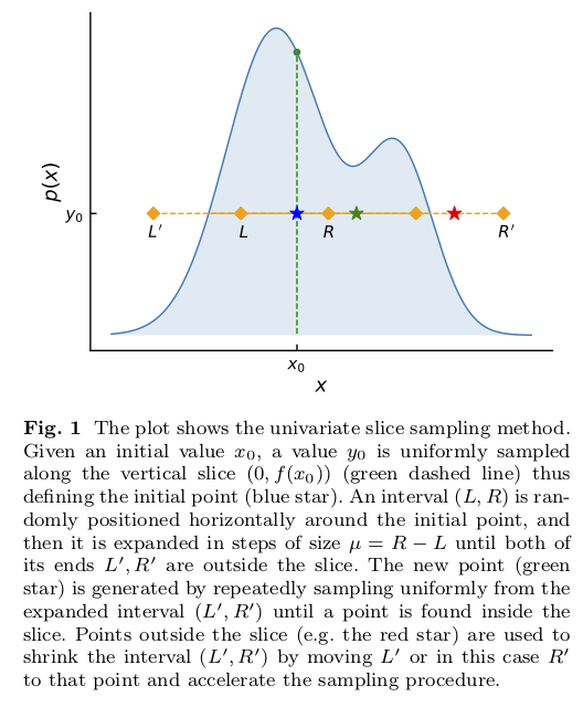
Slice sampling in action for a one-dimensional distribution is shown in Fig. 6.1.
The idea is that sampling from a distribution \(p(x)\) is the same as uniform sampling from the area under the plot of \(f(x) \propto p(x)\). E.g., the highest probability \(p(x)\) is where the area is largest, and this is a simple proportionality. The height \(y\) is introduced with \(0 < y < f(x)\) as an auxiliary variable and one samples the uniform joint probability \(p(x,y)\). Then \(p(x)\) is obtained by marginalizing over \(y\) (meaning just dropping \(y\) from the sample).
The blue star comes from uniformly sampling in \(y\) at the initial point \(x_0\) to identify \(y_0\).
The “slice” is the set of \(x\) such that \(y_0 < f(x)\). In the figure the interval initially from \(L\) to \(R\) is expanded to \(L'\) to \(R'\), which includes the full slice. When the final interval is found, a new \(x_1\) is drawn uniformly from the intersection of the interval and the slice.
The green star is an accepted new point \(x_1\) (inside the slice) while the red star is a rejected point (outside the slice).
There is one parameter to tune: the width \(\mu\) of the interval from \(L\) to \(R\) that sets the original interval around \(x_0\) and then the step size for expanding the interval to be from \(L'\) to \(R'\). In
zeusthe value of \(\mu\) is tuned by stochastic optimization.
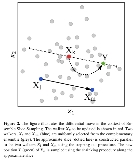
The “ensemble” aspect of zeus is that there are multiple walkers, as in the ensemble sampler emcee.
Figure Fig. 6.2 illustrates how the ensemble of walkers is used to do what is called a “differential move”. There are several choices for moves, including a global one that is effective for multi-modal distributions.
The basic call for
zeuscompared toemceeandPyMC3is illustrated in Comparing samplers for a simple problem.An example from the
zeusdocumentation of sampling from a multimodal distribution is given in zeus: Sampling from multimodal distributions.The text case for parallel tempering in a very simple multi-modal example is compared to
zeusin Example: Parallel tempering for multimodal distributions vs. zeus