3.3. Lecture 8¶

Recap of Poisson MCMC example¶

Notebook: Metropolis-Hasting MCMC sampling of a Poisson distribution

Recall Metropolis algorithm for \(p(\thetavec | D, I)\) (or any other posterior).

start with inital point \(\thetavec_0\) (for each walker)
begin repeat: given \(\thetavec_i\), propose \(\phivec\) from \(q(\phivec|\thetavec_i)\)
calculate \(r\):

\[ r = \frac{p(\phivec|D,I)}{p(\thetavec_i|D,I)} \left[\frac{q(\thetavec_i|\phivec)}{q(\phivec|\thetavec_i)}\right] \]

where the left factor compares posteriors and the right factor is a correction for \(r\) if the \(q\) pdf is not symmetric: \(q(\phivec|\thetavec_i) \neq q(\thetavec_i|\phivec)\)

decide whether to keep \(\phivec\):
- if \(r\geq 1\), set \(\thetavec_{i+1} = \phivec\) (accept)
- else draw \(u \sim \text{uniform}(0,1)\)
  - if \(u \leq r\), \(\thetavec_{i+1} = \phivec\) (accept)
  - else \(\thetavec_{i+1} = \thetavec_i\) (add another copy of \(\thetavec_i\) to the chain)
end repeat when “converged”.

Key questions: When are you converged? How many “warm-up” or “burn-in ” steps to skip?

Poisson take-aways:

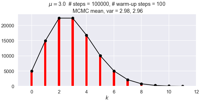
It works! Sampled historgram agrees with (scaled) exact Poisson pdf (that is what success looks like). But not normalized! Compare 1000 to 100,000.
Warm-up time is (apparently) seen from the trace. Moral: always check traces!
The trace also shows that the space is being explored (rather than being confined to one region).
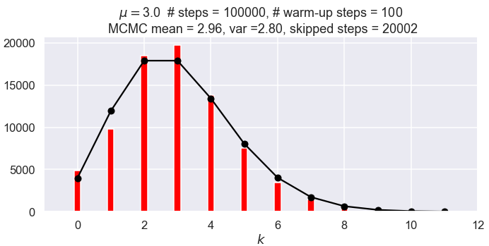
What if the \(\thetavec_{i+1}=\thetavec_i\) step is not implemented as it should be? (I.e., so the chain is only incremented if the step is accepted.) This is not clearly intuitive. But see the figures below with 100,000 steps. The first one follows the Metropolis algorithm and adds the same step if the candidate is rejected; the second one does not. Not keeping the repeated steps invalidates the Markov chain conditions \(\Lra\) wrong stationary distribution (not by a lot but noticeably and every time it is run).
The spread of the means decreases as \(1/\sqrt{N_{\text{steps}}}\), as expected.

Summary points from arXiv:1710.06068

Before considering another example, some summary points from “Data Analysis Recipes: Using Markov Chain Monte Carlo” by David Hogg and Daniel Foreman-Mackey.
- Both are computational astrophysicists (or cosmologists or astronomers)
- DFM wrote emcee.
- Highly experienced in physics scenarios, highly opinionated, but not statisticians (although they interact with statisticians).
MCMC is good for sampling, but not optimizing. If you want to find the modes of distributions, use an optimizer instead.
For MCMC, you only have to calculate ratios of pdfs (as seen from the algorithm).
- \(\Lra\) don’t need analytic normalized pdfs
- \(\Lra\) great for sampling posterior pdfs

\[ p(\thetavec|D) = \frac{1}{Z} p(D|\thetavec)p(\thetavec) \]

Getting \(Z\) is really difficult because you need global information. (Cf. \(Z\) and partition function in statistical mechanics.)
MCMC is extremely easy to implement, without requiring derivatives or integrals of the function (but see later discussion of HMC).
Success means a histogram of the samples looks like the pdf.
Sampling for expectation values works even though we don’t know \(Z\); we just need the set of \(\{\thetavec_k\}\).

\[\begin{split}\begin{align} E_{p(\thetavec)}[\thetavec] &\approx \frac{1}{N}\sum_{k=1}^{N}\thetavec_k \\ E_{p(\thetavec)}[g(\thetavec)] &\approx \frac{1}{N}\sum_{k=1}^{N}g(\thetavec_k) \longrightarrow \frac{\int d\thetavec\, g(\thetavec)f(\thetavec)}{\int d\thetavec\, f(\thetavec)} \end{align}\end{split}\]

where \(f(\thetavec) = Z p(\thetavec)\) is unnormalized.

Nuisance parameters are very easy to marginalize over: just drop that column in every \(\theta_k\).
Autocorrelation is important to monitor and one can tune (e.g., Metropolis step size) to minimize it. More on this later.
How do you know when to stop? Heuristics and diagnostics to come!
Practical advice for initialization and burn-in is given by Hogg and Foreman-Mackey.

MCMC random walk and sampling example¶

Look at the notebook Exercise: Random walk. Let’s do some of the first part together.

Part 1: Random walk in the \([-5,5]\) region. The proposal step is drawn from a normal distribution with zero mean and standard deviation proposal_width.

Algorithm: always accept unless across boundary.

Class: map this problem onto the Metropolis algorithm.

What is \(q(\phivec|\thetavec_i)\)? \(\Lra\) \(\phi \sim \mathcal{N}(\theta_i,(\text{proposal-width})^2)\)

Hint

Use shift-tab-tab to check whether the normal function takes \(\sigma\) or \(\sigma^2\) as an argument.

What is \(p(\thetavec_i|D,I)\)?

It must be constant except for the borders \(\Lra\) \(U(-5,5)\)

Check the answer. Change np.random.seed(10) to np.random.seed()
- This will mean a different pseudo-random number sequence every time you re-run.
- Note the fluctuations.
- Try 200 then 2000 samples.
- Try changing to a uniform proposal.
- Try not adding the rejection position.
Hint

Move samples.append(current_position) under the if statement. Result: it doesn’t fill the full space (try different runs – trouble with edges)
- Decrease width to 0.2, do 2000 steps \(\Lra\) samples are too correlated.
- Look at definition and correlation time for 0.2 and 2.0.
- Trend in autocorrelation plot: 1 at lag \(h=0\); how fast to fluctuations around 0?

Autocorrelation¶

Basic idea: Given a sequence \(Y_t = \{Y_0, Y_1, \ldots\}\) with mean zero, the sequence is uncorrelated if for “lag” \(h>0\), \(Y_t \times Y_{t+h}\) should be equally positive and negative so that we get zero as we average over \(h\). If the mean is not zero, then subtract it first.

We define \(\rho(h)\) by

\[ \rho(h) = \frac{\langle Y_t Y_{t+h}\rangle}{\sqrt{\langle Y_t^2\rangle\langle Y_{t+h}^2\rangle}} , \]

so that \(\rho(h) = 1\) if fully correlated and if uncorrelated \(\rho(h) = 0\). In practice if uncorrelated it will fluctuate around zero with increasing \(h\). It will often be found that \(\rho(h) \propto e^{-h/\tau}\) for \(h < 2\tau\). In terms of a sequence \(X_t\) with nonzero mean \(\Xbar\), we calculate \(\rho(h)\) by sums over when \(X_t\) and \(X_{t+h}\) overlap (“ol”):

\[ \rho(h) = \frac{\sum_{\text{ol}} \bigl[(X_t - \Xbar)(X_{t+h}-\Xbar)\bigr]}{\sqrt{\sum_{\text{ol}} (X_t - \Xbar)^2}\sqrt{\sum_{\text{ol}}(X_{t+h}-\Xbar)^2}} \]

In MCMC chains there will be a typical time until \(\rho(h)\) fluctuates about 0, called the “autocorrelation time”. We’ll return later to look at autocorrelation and related diagnostics.

Intuition for detailed balance and the MH algorithm¶

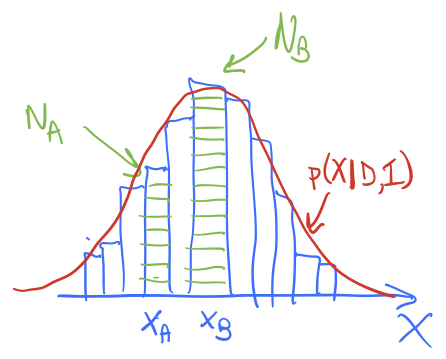
Imagine the schematic histogram here is the accumulated distribution of walkers after some time. The red line is the posterior we are sampling, \(p(X|D,I)\) (we’re using \(X\) instead of \(\thetavec\) for a change of pace), so it is looking like we have an equilibrated distribution (more or less). This doesn’t mean the distribution is static as we continue to sample; walkers will continue to roam around and we’ll accumulate more green boxes at different \(X\) values. But if our Metropolis-Hastings algorithm is correctly implemented, the histogram shape should be stationary at the correct posterior, i.e., it should not change with time except for fluctuations.

Suppose there are \(N_A\) green boxes at \(X_A\) and \(N_B\) green boxes at \(X_B\). With the next Monte Carlo step, each of the boxes at \(X_A\) has a chance to go \(X_B\) while each of the boxes at \(X_B\) has a chance to go to \(X_A\). For a steady-state situation, we want the number of moves in each direction to be the same. (This means that the rates are equal.)

What if the only moves accepted were those that went uphill (i.e., to higher probability density)? What would happen to \(N_A\) and \(N_B\) over time? Is this stationary?

If only uphill move were accepted, then \(N_B\) would monotonically increase while \(N_A\) would eventually monotonically decrease (it would get some input at first from lower probability values of \(X\) but eventually those would all be gone). So all of the boxes would end up at \(x_B\). This is stationary but not at the posterior we are sampling!

Ok, so suppose \(p(X|X')\) is the transition probability, that we’ll move from \(X'\) to \(X\).

In terms of \(p(X_A|X_B)\), \(p(X_B|X_A)\), \(N_A\), and \(N_B\), what is the condition that the exchanges between \(A\) and \(B\) cancel out? (For now assume a symmetric proposal distribution \(q\).)

\[ N_A \cdot p(X_B|X_A) = N_B \cdot p(X_A | X_B) \]

How are \(N_A\) and \(N_B\) related to the total \(N\) and the posteriors \(p(X_A|D,I)\) and \(p(X_B|D,I)\)?

\[ N_A = N \cdot p(X_A|D,I) \qquad N_B = N \cdot p(X_B|D,I) \]

Now let’s put it together.

What is the ratio of \(p(X_B|X_A)\) to \(p(X_A|X_B)\) in terms of \(p(X_A|D,I)\) and \(p(X_B|D,I)\)?

\[ \frac{p(X_B|X_A)}{p(X_A|X_B)} = \frac{N p(X_B|D,I)}{N p(X_A|D,I)} = \frac{p(X_B|D,I)}{p(X_A|D,I)} \]

Now how do we realize a rule that satisfies the condition we just derived? We actually have a lot of freedom in doing so and the Metropolis choice is just one possibility. Let’s verify that it works. The Metropolis algorithm says

\[\begin{split} p(X | X') = \begin{cases} \frac{\displaystyle p(X|D,I)}{\displaystyle p(X'|D,I)} \,, & \text{if } p(X|D,I) \leq p(X'|D,I) \\ 1\,. & \text{if } p(X|D,I) \gt p(X'|D,I) \end{cases} \end{split}\]

Let’s check cases and see if it works. Here is a chart:

	\(p(X_B\vert X_A)\)	\(p(X_A\vert X_B)\)
\(p(X_B\vert D,I) \lt p(X_A\vert D,I)\)	[fill in here]	[fill in here]
\(p(X_A\vert D,I) \lt p(X_B\vert D,I)\)	[fill in here]	[fill in here]

Fill in the chart based on the Metropolis algorithm we are using and verify that the ratio of \(p(X_B|X_A)\) to \(p(X_A|X_B)\) agrees with the answer derived above.

	\(p(X_B\vert X_A)\)	\(p(X_A\vert X_B)\)
\(p(X_B\vert D,I) \lt p(X_A\vert D,I)\)	\(\frac{\displaystyle p(X_B\vert D,I)}{\displaystyle p(X_A\vert D,I)}\)	1
\(p(X_A\vert D,I) \lt p(X_B\vert D,I)\)	1	\(\frac{\displaystyle p(X_A\vert D,I)}{\displaystyle p(X_B\vert D,I)}\)

Dividing the 2nd by the 3rd columns for the 2nd and 3rd rows each gives the correct result!

Ok, so it works. What if we have an asymmetric proposal distribution? So \(q(X|X') \neq q(X'|X)\). Then we just need to go back to where we were equating rates and add the \(q\)s to each side of the equation. The bottom line is the Metropolis algorithm with the Metropolis ratio \(r\) as we have summarized it at the beginning of this lecture.

Why do you think that this property is called detailed balance? Can you make an analogy with thermodynamic equilibrium for e.g. a collection of hydrogen atoms?

You answer!

Learning from data

3.3. Lecture 8¶

Recap of Poisson MCMC example¶

MCMC random walk and sampling example¶

Autocorrelation¶

Intuition for detailed balance and the MH algorithm¶