2.7. Lecture 6¶

Follow-up to priors¶

Return to the discussion of priors for fitting a straight line.

Where does $p(m) \propto 1/(1+m^2)^{3/2}$ come from?
We can consider the line to be given by $y = m x + b$ or $x = m' y + b'$, with $m' = 1/m$ and $b' = -b/m$. These give the same results.
But because the labeling is arbitrary, we expect (and will require) that the prior on $m,b$ (i.e., $p(m,b)$) has the same functional form as those on $m',b'$ (so $p(m',b')$ with the same function $p$). Then for the probabilities, we must have

\[\begin{split} p(m,b)\,dm\,db = p(m', b')\,dm'\,db' = p(1/m,-b/m)\left| \begin{array}{cc} \frac{\partial m'}{\partial m} & \frac{\partial m'}{\partial b} \\ \frac{\partial b'}{\partial m} & \frac{\partial b'}{\partial b} \end{array} \right|\, dm\,db \end{split}\]

Evaluating the Jacobian gives $1/m^3$, so we need to solve the functional equation:

\[ p(1/m, -b/m) = m^3 p(m, b) . \]

A solution is

\[ p(m,b) = \frac{c}{(1 + m^2)^{3/2}} \]

with $c$ chosen to normalize the pdf. Check:

\[ p(1/m, -b/m) = \frac{c}{(1 + (1/m)^2)^{3/2}} = \frac{c}{\frac{1}{m^3}(m^2 + 1)^{3/2}} = m^3 p(m,b) \quad \]

It works! Note that this prior is independent of $b$.

How would you solve this without guessing the answer? Is there more than one solution?

[fill in answer]

Sivia example on “signal on top of background”¶

See [SS06] for further details. The figure shows the set up:

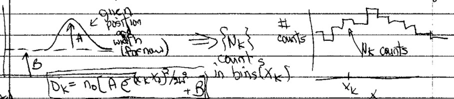
The level of the background is $B$, the peak height of the signal above the background is $A$ and there are $\{N_k\}$ counts in the bins $\{x_k\}$. The distribution is

\[ D_k = n_0 [A e^{-(x_k-x_0)^2/2w^2} + D] \]

Goal: Given $\{N_k\}$, find $A$ and $B$.

So what is the posterior we want?

\[ p(A,B | \{N_k\}, I) \ \mbox{with $I=x_0, w$, Gaussian, flat background} \]

The actual counts we get will be integers, and we can expect a Poisson distribution:

\[ p(n|\mu) = \frac{\mu^n e^-\mu}{n!} \ \mbox{$n\geq 0$ integer} \]

or, with $n\rightarrow N_k$, $\mu \rightarrow D_k$,

\[ p(N_k|D_k) = \frac{D_k e^{-D_k}}{N_k!} \]

for the $k^{\text{th}}$ bin at $x_k$.

What do we learn from the plots of the Poisson distribution?

\[\begin{split}\begin{align} p(A,B | \{N_k\}, I) &\propto p(\{N_k\}|A,B,I) \times p(A,B|I) \\ \textit{posterior}\qquad &\propto \quad\textit{likelihood}\quad \times \quad\textit{prior} \end{align}\end{split}\]

which means that

\[ L = \log[p(A,B)|\{N_k\,I\})] = \text{constant} + \sum_{k=1}^M [N_k \log(D_k) - D_k] \]

Choose the constant for convenience; it is independent of $A,B$.
Best point estimate: maximize $L(A,B)$ to find $A_0,B_0$
Look at code for likelihood and prior
Uniform (flat) prior for $0 \leq A \leq A_{\text{max}}$, $0 < B \leq B_{\text{max}}$
- Not sensitive to $A_{\text{max}}$, $B_{\text{max}}$ if larger than support of likelihood

Table of results

Fig. #	data bins	$\Delta x$	$(x_k)_{\text{max}}$	$D_{\text{max}}$
1	15	1	7	100
2	15	1	7	10
3	31	1	15	100
4	7	1	3	100

Comments on figures:

Figure 1: 15 bins and $D_{\text{max}} = 100$
- Contours are at 20% intervals showing height
- Read off best estimates and compare to true
  - does find signal is about half background
- Marginalization of $B$
  - What if we don’t care about $B$? (“nuisance parameter”)
  \[ p(A | \{N_k\}, I) \int_0^\infty p(A,B|\{N_k\},I)\, dB \]
  - compare to $p(A | \{N_k\}, B_{\text{true}}, I)$ $\Longrightarrow$ plotted on graph
- Also can marginalize over $A$
  
  \[ p(B | \{N_k\}, I) \int_0^\infty p(A,B|\{N_k\},I)\, dA \]
- Note how these are done in code: B_marginalized and B_true_fixed, and note the normalization at the end.
Set extra plots to true
- different representations of the same info and contours in the first three. The last one is an attempt at 68%, 95%, 99.7% (but looks wrong).
- note the difference between contours showing the pdf height and showing the integrated volume.
Look at the other figures and draw conclusions.
How should you design your experiments?
- E.g., how should you bin data, how many counts are needed, what $(x_k)_{\text{max}}$, and so on.

Learning from data

2.7. Lecture 6¶

Follow-up to priors¶

Sivia example on “signal on top of background”¶