3.2. Metropolis-Hasting MCMC sampling of a Poisson distribution¶

This notebook was adapted from Example 1, section 12.2 in Gregory’s Bayesian Logical Data Analysis for the Physical Sciences.

The Poisson discrete random variable from scipy.stats is defined by (see documentation)

\[ p(k|\mu) = \frac{\mu^k e^{-\mu}}{k!} \quad \mbox{for }k\geq 0 \;. \]

where \(k\) is an integer and \(\mu\) is called the shape parameter. The mean and variance of this distribution are both equal to \(\mu\). (Note: Gregory uses a different notation, but we’ll stay consistent with scipy.stats.)

By “sampling a Poisson distribution” we mean we will obtain a set of \(k\) values: \(\{k_1, k_2, k_3, \ldots\}\) that follow this distribution. That is, for a particular \(k_i\), the probability to get that value should be what we get by evaluating \(p(k_i|\mu)\). We know we’ve succeeded if we make a histogram of our set of \(k_i\)s and it looks like \(p(k|\mu)\) (scaled to line up or else our histogram needs to be normalized to one).

The method we’ll use is generically called Markov chain Monte Carlo or MCMC. A Markov chain starts with some initial value, and then each successive value is generated from the previous one. But it is not deterministic: when the new value is chosen, there is a random number involved. The particular version of MCMC used here is called Metropolis-Hasting. You may be familiar with this from a statistical mechanics class, where it is typically applied to the Ising model.

We’ll do the Metropolis-Hasting sampling as follows:

Choose an initial \(k\) (call it \(k_0\)), having already fixed \(\mu\).
Given \(k_i\), sample a uniform random number \(x\) from 0 to 1 (so \(x \sim U(0,1)\)) and propose \(k' = k_i + 1\) if the \(x > 0.5\), otherwise propose \(k' = k_i - 1\).
Compute the Metropolis ratio \(r = p(k'|\mu)\, /\, p(k_i|\mu)\) using the discrete Poisson distribution.
Given another uniform random number \(y \sim U(0,1)\), \(k_{i+1} = k'\) if \(y \leq r\), else \(k_{i+1} = k_i\) (i.e., keep the same value for the next \(k\)).
Repeat 2.-4. until you think you have enough samples of \(k\).
When graphing the posterior or calculating averages, skip the first values until the sampling has equilibrated (this is generally called the “burn-in” or “warm-up”).

In practice we’ll carry this out by generating all our uniform random numbers at the beginning using scipy.stats.uniform.rvs.

%matplotlib inline  

import numpy as np
from math import factorial

# We'll get our uniform distributions from stats, but there are other ways.
import scipy.stats as stats  

import matplotlib.pyplot as plt
import seaborn; seaborn.set() # for nicer plot formatting

def poisson(k, mu):
    """
    Returns a Poisson distribution value for k with mean mu
    """
    return mu**k * np.exp(-mu) / factorial(k) 

In the following we have the steps 1-6 defined above marked in the code. Step through the implementation and ask questions about what you don’t understand.

# 1. Set mu and k0
mu = 3.
k0 = 10    

num_steps = 1000  # number of MCMC steps we'll take
# generate the two sets of uniform random numbers we'll need for 2. and 4.
uniform_1 = stats.uniform.rvs(size=num_steps)  
uniform_2 = stats.uniform.rvs(size=num_steps)

k_array = np.zeros(num_steps, dtype=int)
k_array[0] = k0

# 5. Loop through steps 2-4
for i in range(num_steps-1):  # num_steps-1 so k_array[i+1] is always defined
    # 2. Propose a step
    k_now = k_array[i]
    if uniform_1[i] > 0.5:
        kp = k_now + 1          # step to the right
    else:
        kp = max(0, k_now - 1)  # step to the left, but don't go below zero
    
    # 3. Calculate Metropolis ratio
    metropolis_r = poisson(kp, mu) / poisson(k_now, mu)
    # 4. Accept or reject
    if uniform_2[i] <= metropolis_r:
        k_array[i+1] = kp
    else:
        k_array[i+1] = k_now

# 6. Choose how many steps to skip
warm_up_steps = 100

# Set up for side-by-side plots
fig = plt.figure(figsize=(10,10))

# Plot the trace (that means k_i for i=0 to num_steps)
ax_trace = fig.add_subplot(2, 1, 1)    
ax_trace.plot(range(num_steps), k_array, color='blue')
ax_trace.set_ylim(0, 12)
ax_trace.set_xlabel(r'$i$')
ax_trace.set_ylabel(r'$k_i$')
trace_title = rf'MCMC trace for Poisson distribution with $\mu = ${mu:.1f}'
ax_trace.set_title(trace_title)

# Plot the Poisson distribution
ax_plot = fig.add_subplot(2, 1, 2)
bin_num = 12
n_pts = range(bin_num)
    
# Scale exact result to the histogram, accounting for warm_up_steps    
poisson_pts = [(num_steps - warm_up_steps) * poisson(n, mu) for n in n_pts]     
    
# Plot the exact distribution    
ax_plot.plot(n_pts, poisson_pts, marker='o', color='black') 
# Histogram k_i beyond the warm-up period
ax_plot.hist(k_array[warm_up_steps:], bins=n_pts,
             align='left', rwidth=0.2, color='red')
ax_plot.set_xlim(-1, bin_num)
ax_plot.set_xlabel(r'$k$')
plot_title = rf'$\mu = ${mu:.1f}  # steps = {num_steps:d},' \
               + f' # warm-up steps = {warm_up_steps:d}'
ax_plot.set_title(plot_title)

fig.tight_layout()

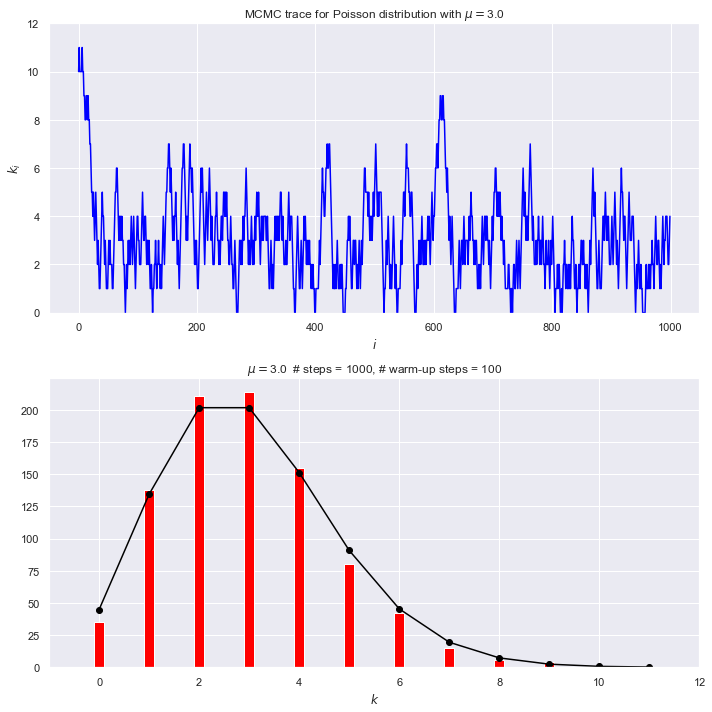
../../_images/Metropolis_Poisson_example_7_0.png

What do you observe about these plots?

# Check the mean and standard deviations from the samples against exact
print(f' MCMC mean = {np.mean(k_array[warm_up_steps:]):.2f}')
print(f'Exact mean = {stats.poisson.mean(mu=mu):.2f}')
print(f'   MCMC sd = {np.std(k_array[warm_up_steps:]):.2f}')
print(f'  Exact sd = {stats.poisson.std(mu=mu):.2f}')      

 MCMC mean = 2.73
Exact mean = 3.00
   MCMC sd = 1.58
  Exact sd = 1.73

Questions and things to do¶

How do you expect the accuracy of the estimate of the mean scales with the number of points? How would you test it?

Record values of the MCMC mean for num_steps = 1000, 4000, and 16000, running each 10-20 times. Explain what you find.

Calculate the mean and standard deviations of the means you found (using np.mean() and np.std()). Explain your results.

Predict what you will find from 10 runs at num_steps = 100,000. What did you actually find?

Learning from data

3.2. Metropolis-Hasting MCMC sampling of a Poisson distribution¶

Questions and things to do¶