2.4. Lecture 5¶

Follow-up to Gaussian approximation

We motivated Gaussian approximations from a Taylor expansion to quadratic order of the logarithm of a pdf. What could go wrong if we directly expanded the pdf?

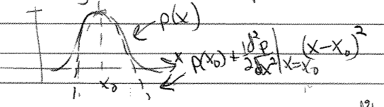
\[ p(x) \approx p(x_0) + \frac{1}{2}-\left.\frac{d^2p}{dx^2}\right|_{x_0}(x-x_0)^2 \ \overset{x\pm\rightarrow\infty}{\longrightarrow} -\infty! \]

A pdf must be normalizable and positive definite, so this approximation violates these conditions!
In contrast,

\[ L(x) = \log p(x) \approx L(x_0) + \frac{1}{2}\left.\frac{d^2L}{dx^2}\right|_{x_0}(x-x_0)^2 \ \Longrightarrow p(x) \approx A e^{\frac{1}{2}\left.\frac{d^2L}{dx^2}\right|_{x_0}(x-x_0)^2} > 0 \]

where we note that the second derivative is less than zero so the exponent is negative definite.

Note that this approximation is not only positive definite and normalizable, it is a higher-order approximation to $p(x)$ because it includes all orders in $(x-x_0)^2$.

Compare Gaussian noise sampling to lighthouse calculation¶

Jump to the Bayesian approach in Parameter estimation example: Gaussian noise and averages and then come back to contrast with the frequentist approach.
Compare the goals between the Gaussian noise sampling (left) and the radioactive lighthouse problem (right): in both cases the goal is to sample a posterior $p(\thetavec|D,I)$

\[ p(\mu,\sigma | D, I) \leftrightarrow p(x_0,y_0 | D, I) \]

where $D$ on the left are the $x$ points and $D$ on the right are the $\{x_k\}$ where flashes hit.
What do we need? From Bayes’ theorem, we need

\[\begin{split}\begin{align} \text{likelihood:}& \quad p(D|\mu,\sigma,I) \leftrightarrow p(D|x_0,y_0,I) \\ \text{prior:}& \quad p(\mu,\sigma|I) \leftrightarrow p(x_0,y_0|I) \end{align}\end{split}\]
You are generalizing the functions for log pdfs and the plotting of posteriors that are in notebook Radioactive lighthouse problem Key.
Note in Parameter estimation example: Gaussian noise and averages the functions for log-prior and log-likelihood.
- Here $\thetavec = [\mu,\sigma]$ is a vector of parameters; cf. $\thetavec = [x_0,y_0]$.
Step through the set up for emcee.
- It is best to create an environment that will include emcee and corner.
Hint

Nothing in the emcee sampling part needs to change!
- More later on what is happening, but basically we are doing 50 random walks in parallel to explore the posterior. Where the walkers end up will define our samples of $\mu,\sigma$ $\Longrightarrow$ the histogram is an approximation to the (unnormalized) joint posterior.
- Plotting is also the same, once you change labels and mu_true, sigma_true to x0_true, y0_true. (And skip the maxlike part.)
Analysis:
- Maximum likelihood here is the frequentist estimate $\longrightarrow$ this is an optimization problem.
Question

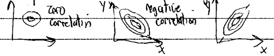
Are $\mu$ and $\sigma$ correlated or uncorrelated?

Answer

They are uncorrelated because the contour ellipses in the joint posterior have their major and minor axes parallel to the $\mu$ and $\sigma$ axes. Note that the fact that they look like circles is just an accident of the ranges chosen for the axes; if you changed the $\sigma$ axis range by a factor of two, the circle would become flattened.
- Read off marginalized estimates for $\mu$ and $\sigma$.

Central limit theorem (CLT)¶

Let’s start with a general characterization of the central limit theorem (CLT):

General form of the CLT

The sum of $n$ random variables that are drawn from any pdf(s) of finite variance $\sigma^2$ tends as $n\rightarrow\infty$ to be Gaussian distributed about the expectation value of the sum, with variance $n\sigma^2$. (So we scale the sum by $1/\sqrt{n}$; see below.)

Consequences:

The mean of a large number of values becomes normally distributed regardless of the probability distribution from which the values are drawn. (Why does this fail for the lighthouse problem?)
Functions such as the Binomial and Poisson distribution all tend to Gaussian distributions with a large number of draws.

\[ \text{E.g., } P_n = \frac{\lambda^n e^{-\lambda}}{n!} %\ \mbox{($n$ an integer)}\ \overset{\lambda\rightarrow\text{large}}{\underset{n\rightarrow x\rightarrow\text{large}}{\longrightarrow}} p(x) = \frac{e^{-(x-\lambda)^2/2\lambda}}{\sqrt{2\pi\lambda}} \]

so mean $\mu = \lambda$ and variance $\sigma^2 = \lambda$ (variance, not the standard deviation).

Class questions

i) How would you verify this in a Jupyter notebook?
ii) How would you prove it analytically?

Answer

[add an answer]

Proof in special case¶

Start with independent random variables $x_1,\cdots,x_n$ drawn from a distribution with mean $\langle x \rangle = 0$ and variance $\langle x^2\rangle = \sigma^2$, where

\[ \langle x^n \rangle \equiv \int x^n p(x)\, dx \]

(generalize later to nonzero mean). Now let

\[ X = \frac{1}{\sqrt{n}}(x_1 + x_2 + \cdots + x_n) = \sum_{j=1}^n \frac{x_j}{\sqrt{n}} , \]

(we scale by $1/\sqrt{n}$ so that $X$ is finite in the $n\rightarrow\infty$ limit).

What is the distribution of $X$? $\Longrightarrow$ call it $p(X|I)$, where $I$ is the information about the probability distribution for $x_j$.

Plan: Use the sum and product rules and their consequences to relate $p(X)$ to what we know of $p(x_j)$. (Note: we’ll suppress $I$ to keep the formulas from getting too cluttered.)

\[\begin{split}\begin{align} p(X) &= \int_{-\infty}^{\infty} dx_1 \cdots dx_n\, p(X,x_1,\cdots,x_n) \\ &= \int_{-\infty}^{\infty} dx_1 \cdots dx_n\, p(X|x_1,\cdots,x_n)\,p(x_1,\cdots,x_n) \\ &= \int_{-\infty}^{\infty} dx_1 \cdots dx_n\, p(X|x_1,\cdots,x_n)\,p(x_1)\cdots p(x_n) . \end{align}\end{split}\]

Class: state the rule used to justify each step

marginalization
product rule
independence

We might proceed by using a direct, normalized expression for $p(X|x_1,\cdots,x_n)$:

Question

What is $p(X|x_1,\cdots,x_n)$?

Answer

$p(X|x_1,\cdots,x_n) = \delta\Bigl(X - \frac{1}{\sqrt{n}}(x_1 + \cdots + x_n)\Bigr)$

Instead we will use a Fourier representation:

\[ p(X|x_1,\cdots,x_n) = \delta\Bigl(X - \frac{1}{\sqrt{n}}(x_1 + \cdots + x_n)\Bigr) = \frac{1}{2\pi} \int_{-\infty}^{\infty} d\omega \, e^{i\omega\Bigl(X - \frac{1}{\sqrt{n}}\sum_{j=1}^n x_j\Bigr)} . \]

Substituting into $p(X)$ and gathering together all pieces with $x_j$ dependence while exchanging the order of integrations:

\[ p(X) = \frac{1}{2\pi} \int_{-\infty}^{\infty} d\omega \, e^{i\omega X} \prod_{j=1}^n \left[\int_{-\infty}^{\infty} dx_j\, e^{i\omega x_j / \sqrt{n}} p(x_j) \right] \]

Observe that the terms in []s have factorized into a product of independent integrals and they are all the same (just different labels for the integration variables).
Now we Taylor expand $e^{i\omega x_j/\sqrt{n}}$, arguing that the Fourier integral is dominated by small $x$ as $n\rightarrow\infty$. (When does this fail?)

\[ e^{i\omega x/\sqrt{n}} = 1 + \frac{i\omega x}{\sqrt{n}} + \frac{(i\omega)^2 x^2}{2 n} + \mathcal{O}\left(\frac{\omega^3 x^3}{n^{3/2}}\right) \]

Then, using that $p(x)$ is normalized (i.e., $\int_{-\infty}^{\infty} dx\, p(x) = 1$),

\[\begin{split}\begin{align} \int_{-\infty}^{\infty} dx\, e^{i\omega x / \sqrt{n}} p(x) &= \int_{-\infty}^{\infty} dx\, p(x) \left[ 1 + \frac{i\omega x}{\sqrt{n}} + \frac{(i\omega)^2 x^2}{2n} + \cdots \right] \\ &= 1 + \frac{i\omega}{\sqrt{n}}\langle x \rangle - \frac{\omega^2}{2n} \langle x^2 \rangle + \langle x^3 \rangle \mathcal{O}\left(\frac{\omega^3}{n^{3/2}}\right) \\ &= 1 - \frac{\omega^2 \sigma^2}{2n} + \mathcal{O}\left(\frac{\omega^3}{n^{3/2}}\right) \qquad [\langle x\rangle = 0 \text{ by assumption}] \end{align}\end{split}\]

Now we can substitute into the posterior for $X$ and take the large $n$ limit:

\[\begin{split}\begin{align} p(X) &= \frac{1}{2\pi} \int_{-\infty}^{\infty} d\omega \, e^{i\omega X} \left[1 - \frac{\omega^2 \sigma^2}{2n} + \mathcal{O}\left(\frac{\omega^3}{n^{3/2}}\right)\right]^n \\ &\overset{n\rightarrow\infty}{\longrightarrow} \frac{1}{2\pi} \int_{-\infty}^{\infty} d\omega \, e^{i\omega X} e^{-\omega^2\sigma^2/2} = \frac{1}{\sqrt{2\pi}} e^{-X^2/2\sigma^2} \quad \text{QED} \end{align}\end{split}\]

Here we’ve used:

$\lim_{n\rightarrow\infty}\left(1+\frac{a}{n}\right)^n = e^a$ with $a = -\omega^2\sigma^2/2$.
$\int_{-\infty}^{\infty} dz\, e^{-Az^2/2}e^{iBz} = \sqrt{2\pi/A} e^{-B^2/2A}$ with $z = \omega$, $A = \sigma^2$, and $B = X$.

To generalize to $\langle x \rangle \neq 0$ (non-zero mean), consider $X = \bigl[(x_1 + \cdots x_n) - n\mu\bigr]/\sqrt{n}$ and change to $y_j = x_j - \mu$. Now $X$ is a sum of $y_j$’s and the proof goes through the same.
So the distribution of means of samples of size $n$ from any distribution with finite variance becomes for large $n$ a Gaussian with width equal to the standard deviation of the distribution divided by $\sqrt{n}$.

Correlated posteriors¶

The pdfs we’ve seen for $p(\mu,\sigma|D,I)$ were characterized by elliptical contours of equal probability density whose major axes are aligned with the $\mu$ and $\sigma$ axes.
- We have commented that this is a signal of independent random variables.
- Let’s look at a case where this is not true and then look analytically at what we should expect with correlations.
So return to notebook Parameter estimation example: fitting a straight line
- Review the statistical model.
- What are we trying to find? $p(\thetavec|D,I)$, just as in the other notebooks, now with $\thetavec =[b,m]$.

Comments on the notebook:

Note that $x_i$ is alo randomly distributed uniformly.
Log likelihood gives fluctuating results whose size depend on the # of data points $N$ and the standard deviation of the noise $dy$.

Explore!

Play with the notebook and explore how the size varies with $N$ and $dy$.

Compare priors on the slope $\Longrightarrow$ uniform in $m$ vs. uniform in angle.
Implementation of plots comparing priors:

Questions for the class

With the first set of data with $N=20$ points, does the prior matter?
With the second set of data with $N=3$ points, does the prior matter?

Answers

No!
Yes!

Note: log(posterior) = log(likelihood) + log(prior)
- Maximum is set to 1 for plotting
- Exponentiate: posterior = exp(log(posterior))

What does it mean that the ellipses are slanted?

On the second set of data:
- True answers are intercept $b = 25.0$, slope $m=0.5$.
- Flat prior gives $b = -50 \pm 75$, $m = 1.5 \pm 1, so barely at the $1\sigma$ level.
- Symmetric prior gives $b = 25 \pm 50$, slope = 0.5 \pm 0.75, so much better.
- Distributions are wide (only three points!).

Likelihoods (or posteriors) with two variables with quadratic approximation¶

Find $X_0$, $Y_0$ (best estimate) by differentiating

\[\begin{split}\begin{align} L(X,Y) &= \log p(X,Y|\{\text{data}\}, I) \\ \quad&\Longrightarrow\quad \left.\frac{dL}{dX}\right|_{X_0,Y_0} = 0, \ \left.\frac{dL}{dY}\right|_{X_0,Y_0} = 0 \end{align}\end{split}\]

To check reliability, Taylor expand around $L(X_0,Y_0)$:

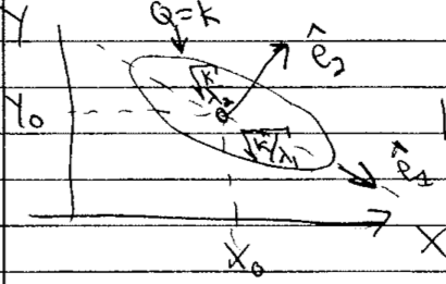
\[\begin{split}\begin{align} L &= L(X_0,Y_0) + \frac{1}{2}\Bigl[ \left.\frac{\partial^2L}{\partial X^2}\right|_{X_0,Y_0}(X-X_0)^2 + \left.\frac{\partial^2L}{\partial Y^2}\right|_{X_0,Y_0}(Y-Y_0)^2 \\ & \qquad\qquad\qquad + 2 \left.\frac{\partial^2L}{\partial X\partial Y}\right|_{X_0,Y_0}(X-X_0)(Y-Y_0) \Bigr] + \ldots \\ &\equiv L(X_0, Y_0) + \frac{1}{2}Q + \ldots \end{align}\end{split}\]

It makes sense to do this in (symmetric) matrix notation:

\[\begin{split} Q = \begin{pmatrix} X-X_0 & Y-Y_0 \end{pmatrix} \begin{pmatrix} A & C \\ C & B \end{pmatrix} \begin{pmatrix} X-X_0 \\ Y-Y_0 \end{pmatrix} \end{split}\]

\[ \Longrightarrow A = \left.\frac{\partial^2L}{\partial X^2}\right|_{X_0,Y_0}, \quad B = \left.\frac{\partial^2L}{\partial Y^2}\right|_{X_0,Y_0}, \quad C = \left.\frac{\partial^2L}{\partial X\partial Y}\right|_{X_0,Y_0} \]

So in quadratic approximation, the contour $Q=k$ for some $k$ is an ellipse centered at $X_0, Y_0$. The orientation and eccentricity are determined by $A$, $B$, and $C$.
The principal axes are found from the eigenvectors of the Hessian matrix $\begin{pmatrix} A & C \\ C & B \end{pmatrix}$.

\[\begin{split} \begin{pmatrix} A & C \\ C & B \end{pmatrix} \begin{pmatrix} x \\ y \end{pmatrix} = \lambda \begin{pmatrix} x \\ y \end{pmatrix} \quad\Longrightarrow\quad \lambda_1,\lambda_2 < 0 \ \mbox{so $(x_0,y_0)$ is a maximum} \end{split}\]

What is the ellipse is skewed?

Look at correlation matrix

\[\begin{split} \begin{pmatrix} \sigma_x^2 & \sigma^2_{xy} \\ \sigma^2_{xy} & \sigma_y^2 \end{pmatrix} = - \begin{pmatrix} A & C \\ C & B \end{pmatrix}^{-1} \end{split}\]

Learning from data