6.1. Lecture 17¶

Parallel tempering summary points¶

Simulate $N$ replicas of a system at different $\beta = 1/T$, where the temperature dependent log posterior is

\[ \log p_\beta(\thetavec|D,I) = C + \beta \log p(D|\thetavec,I) + \log p(\thetavec|I) . \]
- The temperatures range from $\beta$ small ($T$ large) to $\beta = 1$, which is the results we are trying to find. The user chooses the $\beta$ values.
- $\beta = 0$ samples the prior, so it is spread over the accessible parameter space.
- As $\beta$ ranges from 0 to 1, the impact of the likelihood increases, so that the details in the posterior emerge.
The $N$ chains run in parallel. A swap of configurations is proposed at random intervals between adjacent chains. A Metropolis-like criterion is used to decide whether the swap is selected or not.
The evidence (or marginal likelihood) for model $M$,

\[ p(D|M,I) = \int p(D|\thetavec,M,I) p(\thetavec|M,I)\,d\thetavec , \]

can be calculated numerically by thermodynamic integration using the results at all the temperatures in a numerical quadrature formula. Other approaches for the Bayes factor (ratio of evidences) are discussed in Computing Bayes Factors.

Why not simply calculate the evidence directly?

In some cases we can calculate the evidence directly. If a conjugate prior applies (the likelihood and prior are such that the posterior is the same type of distribution as the prior), we can get an exact result analytically. Or we can approximate using Laplace’s method, which expands the log likelihood around the peak to quadratic order, leaving an analytic Gaussian integral. (For this approximation to a normal distribution you need the mode and the covariance matrix, both obtainable by sampling or, more accurately, by optimization.)

Several reasons make a direct numerical calculation of the evidence difficult:

The dimensionality of the integral required to evaluate the evidence can be high since it is equal to the number of parameters in the model under consideration.
The integrand often has one or more very large and very narrow peaks so that a few small regions of the parameter space contribute most of the integral’s value.
For some problems the dynamic range of the evidence is sufficiently large so that only the log of the evidence can be expressed as a floating-point number. In this case the likelihoods cannot be evaluated using the standard expressions.

Note that it doesn’t help to have our $N$ MCMC samples $\{\thetavec_i\}$, $i = 1,\ldots,N$ of the posterior. We are able to get properly normalized expectation values because of the approximation of the posterior as a sum of $d$-dimensional delta functions ($d$ is the number of parameters in $\thetavec$):

\[ p(\thetavec|D,I) \approx \frac{1}{N}\sum_{i=1}^{N}\delta^d( \thetavec - \thetavec_i) \quad\Lra\quad \langle f(\thetavec) \rangle \approx \frac{1}{N}\sum_{i=1}^{N} f(\thetavec_i) . \]

But this doesn’t help to get the normalization integral of the likelihood times the prior. We can evaluate the evidence as the expectation value of the likelihood with MCMC samples of the prior. This “naive” approach will not generally be robust.

Note on $\chi^2/\text{dof}$ for model assessment and comparison¶

Many physicists learn to judge whether a fit of a model to data is good or to pick out the best fitting model among several by evaluating the $\chi^2/\text{dof}$ for a given model and comparing the result to one. Here $\chi^2$ is the sum of the squares of the residuals (data minus model predictions) divided by variance of the error at each point:

\[ \chi^2 \equiv \sum_{i=1}^{N_{\text{data}}} \frac{\bigl(y_i - f(x_i;\hat\thetavec)\bigr)^2}{\sigma_i^2} , \]

where $y_i$ is the $i^{\text th}$ data point, $f(x_i;\hat\thetavec)$ is the prediction of the model for that point using the best fit for the parameters, $\hat\thetavec$, and $\sigma_i$ is the error bar for that data point. The degrees-of-freedom (dof), often denoted by $\nu$, is the number of data points minus number of fitted parameters:

(6.1)¶\[ \nu = N_{\text{data}} - N_{\text{fit parameters}} . \]

The rule of thumb is generally that $\chi^2 \gg 1$ means a poor fit and $\chi^2 < 1$ indicates overfitting. Where does this come from and under what conditions is it a statistically valid thing to analyze fit models this way? (Note that in contrast to the Bayesian evidence, we are not assessing the model in general, but a particular fit to the model.)

Underlying this use of $\chi^2/\text{dof}$ is a particular, familiar statistical model

\[ y_{\text expt} = y_{\text th} + \delta y_{\text expt} + \delta y_{\text th} \]

in which the theory is $y_{{\text th},i} = f(x_i;\hat\thetavec)$, the experimental error is independent Gaussian distributed noise with mean zero and standard deviation $\sigma_i$, that is $\delta y_{\text expt} \sim \mathcal{N}(0,\Sigma)$ with $\Sigma_{ij} = \sigma_i^2 \delta_{ij}$, and $\delta y_{\text th}$ is neglected (i.e., no model discrepancy is included). The prior is (usually implicitly) taken to be uniform, so

\[ y_{\text expt} \sim \mathcal{N}\bigl(f(x_i;\hat\thetavec), \Sigma\bigr) . \]

The likelihood (and the posterior, with a uniform prior) is then proportional to $e^{-\chi^2(\hat\thetavec)/2}$.

According to this model, each squared term in $\chi^2$ is drawn from a standard normal distribution. In this context, “standard” means that the distribution has mean zero and variance 1. This is exactly what happens when we take as the random variables $\bigl(y_i - f(x_i;\hat\thetavec)\bigr)/\sigma_i$. But the sum of the squares of $k$ independent standard normal random variables has a known distribution, called the $\chi^2$ distribution with $k$ degrees of freedom. So the sum of the normalized residuals squared should be distributed (if you generated many sets of them) as a $\chi^2$ distribution. How many degrees of freedom? This should be the number of independent pieces of information. But we have found the fitted parameters $\hat\thetavec$ by minimizing $\chi^2$, i.e., by setting $\partial \chi^2(\thetavec)/\partial \theta_j$ for $j = 1,\ldots,N_{\text{fit parameters}}$, which means $N_{\text{fit parameters}}$ constraints. Therefore the number of dofs is given by $\nu$ in (6.1).

Now what do we do with this information? We only have one draw from the (supposed) $\chi^2$ distribution. But if that distribution is narrow, we should be close to the mean. The mean of a $\chi^2$ distribution with $k = \nu$ dofs is $\nu$, with variance $2\nu$. So if we’ve got a good fit (and our statistical model is valid), then $\chi^2/\nu$ should be close to one. If it is much larger, than the conditions are not satisfied, so the model doesn’t work. If it is smaller, than the failure implies that the residuals are too small, meaning overfitting.

But we should expect fluctuations, i.e., we shouldn’t always get the mean (or the mode, which is $\nu - 2$ for $\nu\geq 0$). If $\nu$ is large enough, then the distribution is approximately Gaussian and we can use the standard deviation / dof or $\sqrt{2\nu}/\nu = \sqrt{2/\nu}$ as an expected width around one. One might use two or three times $\sigma$ as a range to consider. If there are 1000 data points, then $\sigma \approx 0.045$, so $0.91 \leq \chi^2/\text{dof} \leq 1.09$ would be an acceptable range at the 95% confidence level ($2\sigma$). With fewer data points this range grows significantly. So in making the comparison of $\chi^2/\nu$ to one, be sure to take into account the width of the distribution, i.e., consider $\pm \sqrt{2/\nu}$ roughly. For a small number of data points, do a better analysis!

What can go wrong? Lots! See “Do’s and Don’ts of reduced chi-squared” for a thorough discussion. But we’ve assumed that the data is Gaussian and independent, that data is dominated by experimental and not theoretical errors, and that the constraints from fitting are linearly independent. We’ve also assumed a lot of data and we’ve ignored informative (or, more precisely, non-uniform priors) priors.

Overview of Mini-project IIb: How many lines?¶

The notebook for Mini-project IIb is Mini-project IIb: How many lines are there?.

The problem is adapted from Sivia, section 4.2.
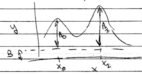
Basic problem: we are given a noisy spectrum (maybe it is intensity as a function of frequency of electromagnetic signals) with some number of signal lines along with background signals. We want to use parameter estimation and model selection (via parallel tempering) to determine what we can about the peaks.
- Model selection addresses how many peaks;
- parameter estimation addresses what are the positions and amplitudes of the peaks.
The true (i.e., underlying) model is a sum of Gaussians plus a constant background.
- The knowledge you have to analyze the data is the known width of the Gaussians but not how many Gaussians there are, nor what their amplitudes and positions are.
- We add Gaussian noise with known $\sigma_{\text{exp}}$ to each data point.
- If there are $M$ lines, then there are $2M+1$ model parameters $\alphavec = (A_0, x_0, A_1, x_1, \ldots, B)$.
- Formulas are in the notebook.

Handdrawn schematic of the underlying model

There are 5 required subtasks, plus a bonus subtask and one to do to get a plus. Some notes:
1. Formulate the problem in Bayesian language of how many lines and what are the model parameters.
  - This amounts to working through Sivia 4.2.
2. Derive an approximation for the posterior probability.
  - Again, Sivia 4.2 has intermediate steps, but try doing it yourself. Be careful of the $M$!
  - Where is the Ockham factor?
  - Does this assume $B$ is known?
3. Optional: numerical implementation.
4. Generate data $\Lra$ just need to look at fluctuations and impact of width and noise.
5. Parameter estimation with emcee.
  - Show what happens with numpeaks = 2.
  - Your job: explain!
6. Main part: parallel tempering (with ptemcee) results for the evidence.
  - Explain the behavior (clear maximum or saturation).
  - Connect to toy model results.
7. Repeat for another situation (different # of peaks, width, or noise).

Hamiltonian Monte Carlo (HMC) overview and visualization¶

We’ve seen some different strategies for sampling difficult posteriors, such as an affine-invariant sampling approach (emcee) and a thermodynamic approach (parallel tempering).
One of the most widespread techniques in contemporary samplers is Hamiltonian Monte Carlo, or HMC.
- We’ll look at some visualizations as motivation, then consider some examples using PyMC3.
We return to the excellent set of interactive demos by Chi Feng at https://chi-feng.github.io/mcmc-demo/ and their adaptation by Richard McElreath at http://elevanth.org/blog/2017/11/28/build-a-better-markov-chain/. These are also linked on the 8820 Carmen visualization page.
The McElreath blog piece forcefully advocates abandoning Metropolis-Hasting (MH) sampling in favor of HMC. Let’s take a look.
- First recall the random walk MH:
  1. Make a random proposal for new parameter values (a step in parameter space, indicated in the visualization by an arrow).
  2. Aceept (green arrow) or reject (red arrow) based on a Metropolis criterion (which is not deterministic but has a random element).
- This is diffusion (i.e., a random walk), so it is not efficient in exploring the parameter space and needs special tuning to avoid too high a rejection rate.
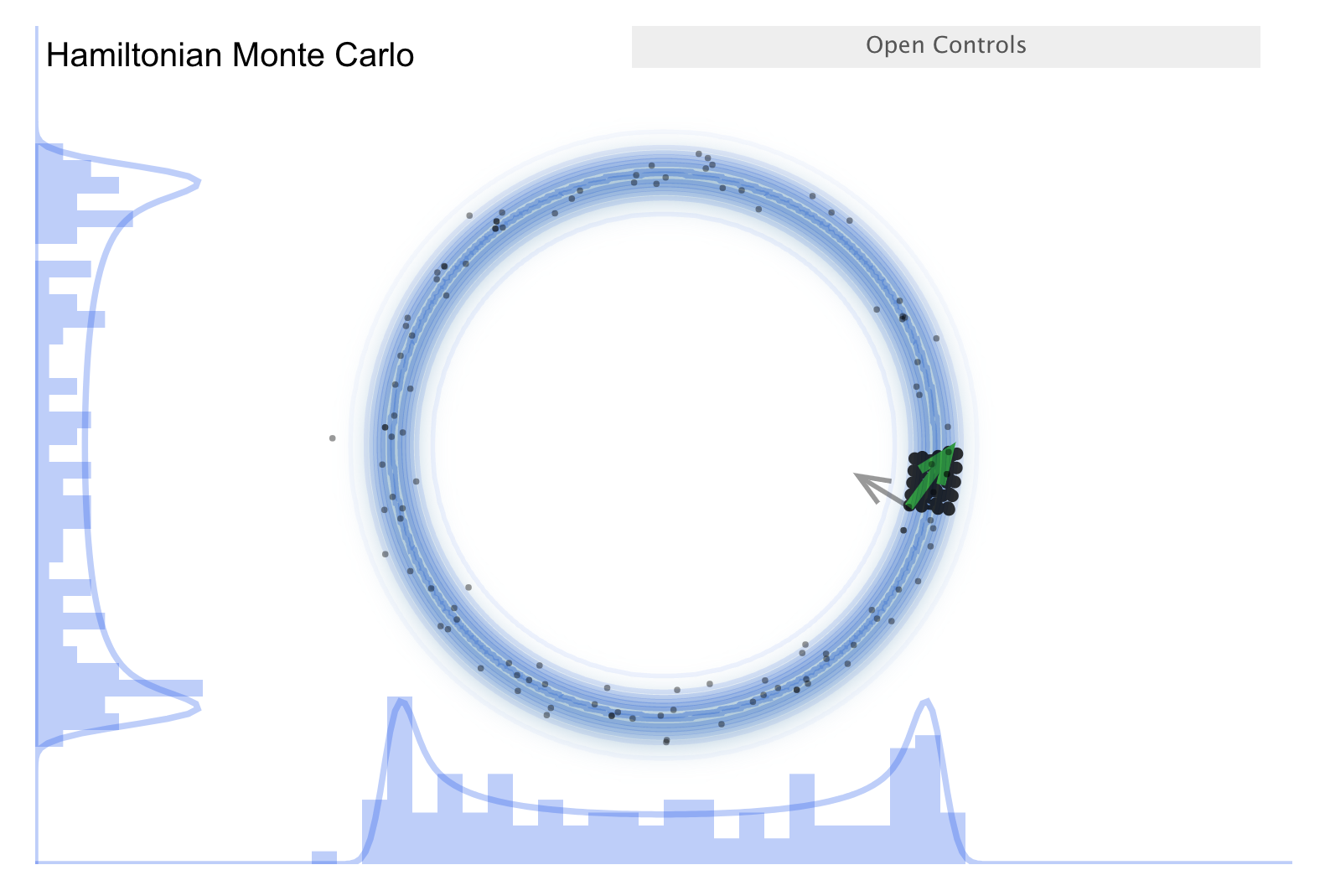
- The donut shape in the simulation is common in higher dimensions and it is difficult to explore. (I.e., consider a multidimensional uncorrelated Gaussian distribution. In spherical coordinates the distribution is $\propto r^n e^{-r^2/2\sigma^2}$, so the marginalized distribution will be peaked away from $r=0$.)
Now consider the “Better living through Physics” part $\Lra$ an HMC simulation.
- The idea is that we map our parameter vector $\thetavec$ of length $n$ to a particle in an $n$-dimensional space. The surface is an $n$-dimensional (inverted) bowl with the shape given by minus-log(target distribution), where the target distribution is the posterior.
- Treat the system as frictionless. “Flick” the particle in a random direction, so it travels across the bowl.
- See the simulation: the little gray arrow is the flick. After the particle travels some distance, decide whether to accept. Most endpoints are within a high probability region, so a high percentage is accepted.
- Chains can get far from the starting point easily $\Lra$ efficient exploration of the full shape.
- More calculation along the path is needed, but fewer samples $\Lra$ this is typically a winning trade-off.
- Check the donut example $\Lra$ works very well!

There is a further improvement called NUTS, which stands for “no-U-turn sampler”.
- The idea is to address the problem that HMV needs to be told how many steps to take before another random flick.
- Too few steps $\Lra$ samples are too similar
- Too many steps $\Lra$ also too similar
NUTS adaptively finds a good number of steps.
- Simulates in *both$ directions to figure out when the path turns around (U-turns) and stops there.
- There are other adaptive features - see the documentation.
Note that NUTS still has trouble with multimodal targets $\Lra$ can explore each high probability area, but has trouble going between them.

HMC physics¶

The basic idea behind HMC is to translate a pdf for the desired distribution into a postential energy function and to add a (fictitious!) momentum variable. In the Markov chain at each iteration, one resamples the momentum (the flick!), creates a proposal using classical Hamiltonian dynamics, and then does a Metropolis update.
Recall Hamiltonian dynamics, now applied to a $d$-dimensional position vector $q$ and a $d$-dimensional momentum vector $p$ $\Lra$ there is a $2\times d$-dimensional phase space for the Hamiltonian $H(q,p)$.
The Hamilton equations of motion describe the time evolution:

\[ \frac{dq_i}{dt} = \frac{\partial H}{\partial p_i}, \qquad \frac{dp_i}{dt} = -\frac{\partial H}{\partial q_i}, \quad i = 1,\ldots d , \]

which map states at time $t$ to states at time $t+s$. (Recall the difference between total and partial derivaties; e.g., what is held fixed in each case.)

We take the form of $H$ to be $H(q,p) = U(q) + K(p)$
- the potential energy $U(q)$ is minus the log probability density of the distribution for $q$ that we seek to sample.
- $K(p)$ is the kinetic energy
\[ K(p) = \frac{1}{2}p^\intercal M^{-1} p , \]

where $M$ is a symmetic, positive (what does that mean?) “mass matrix”, typically diagonal and even $M\times \mathbb{1}_d$ (proportional to the identity matrix in $d$-dimensions).
- This is minus the log probability density (plus a constant) of a Gaussian with zero mean and covariance matrix $M$.
What are we going to do with this? We consider a canonical distribution at temperature $T$:

\[ P(q,p) = \frac{1}{Z} e^{-H(q,p)/T} = \frac{1}{Z} e^{-U(q)/T}e^{-K(p)/T} , \]

so $q$ and $p$ are independent. We are interested only $q$; $p$ is a fake variable to make things work. Usually $U(q)$ is a posterior: $U(q) = -\log[p(q|D)p(q)]$ where $q \rightarrow \thetavec$.

HMC algorithm¶

Two steps of the HMC algorithm:

New values for the momentum variables are randomly drawn from their Gaussian distribution, independent of current position values.
- This means $p_i$ will have mean zero and variance $M_{ii}$ if $M$ is diagonal.
- $q$ isn’t changed, $p$ is from the correct conditional distribution given $q$, so the canonical joint distribution is invariant.
Proposal from Hamiltonian dynamics for a new state. Simulate from $(q,p)$ with $L$ steps of size $\epsilon$. At the end, the momenta are flipped in sign and the new proposed step $(q^*,p^*)$ is accepted with probability (cf. $\Delta E$ with $T=1$):

\[ \min[1,e^{-H(q^*,p^*) + H(q,p)}] = \min[1,e^{-U(q^*)+U(q)-K(p^*)+K(p)}] . \]
- The momentum flip makes the proposal symmetric, but not done in practice.
- So the probability distribution for $(q,p)$ jointly is (almost) unchanged because energy is conserved, but in terms of $q$ we get a very different probability density.

You can show that HMC leaves the canonical distribution invariant because detailed balance holds, which is what we need. It will also be ergodic $\Lra$ it doesn’t get stuck in a subset of phase space but samples all of it.
Essential features:
- Reversability needed so that desired distribution is invariant.
- Conservation of the Hamiltonian (which is the energy here).
- Volume preservation - preserves volume in $(q,p)$ phase space - this is Liouville’s Theorem. (If we take a cluster of points and follow their time evolution, the volume they occupy is unchanged. See Liouville Theorem Visualization notebook.) $\Lra$ this is critical because a change in volume would mean we would have to make a nontreival adjustment to the proposal (because the normalization $Z$ would change).
These requirements are satisfied by the exact Hamilton’s equations, but we are approximating the solution to these differential equations. This necessitates a symplectic (symmetry conserving) integration.
- Ordinary Runge-Kutta-type ODE solvers won’t work because they are not time-reversal invariant.
- E.g., consider the Euler method. Forward and backward integrations are different because the derivatives are calculated from different points.
- We need something like the Leapfrog algorithm (2nd order version here):
\[\begin{split}\begin{align} p_i(t+\epsilon/2) &= p_i(t) - \frac{\epsilon}{2}\frac{\partial U}{\partial q_i}\bigl(q(t)\bigr) \quad \longleftarrow\text{half step} \\ q_i(t+\epsilon) &= q_i(t) + \epsilon p_i(t + \epsilon/2)/M_i \quad\longleftarrow\text{use intermediate $p$} \\ p_i(t+\epsilon) &= p_i(t+\epsilon/2) - \frac{\epsilon}{2}\frac{\partial U}{\partial q_i}\bigl(q(t+\epsilon)\bigr) \quad \longleftarrow\text{other half step} \\ \end{align}\end{split}\]

See Figures 1, and 3-6 in “MCMC using Hamiltonian dynamics” by Radford Neal.

Learning from data