9.1. Lecture 22
MaxEnt function reconstruction
Quick summary of Maximum Entropy for reconstructing a function from its moments:
Consider a function \(f(x)\) on \(x \in [0,1]\) with \(f(x)>0\), i.e., like a probability distribution, and without loss of generality we can assume that \(f(x)\) is normalized (just an overall constant). Suppose we know moments \(\mu_j\) of the function:
(9.1)¶\[ \mu_j = \int_0^1 dx \, x^j f(x), \quad j=0,\ldots,N . \]Our goal is to best reconstruct \(f(x)\) from the \(N+1\) moments. This seems problematic as there are an infinite number of different functions that share that set of moments. Here we use maximum entropy as a prescription for the construction of a sequence of approximations, one for each \(N\), which converges to \(f(x)\) as \(N\rightarrow \infty\).
As before, we define the entropy functional
\[ S[f] = -\int_0^1 dx\, \bigl(f(x)\log f(x) - f(x) \bigr) + \sum_{j=0}^N \lambda_j \left(\int_{0}^{1} dx\, x^j f(x) - \mu_j\right) , \]where the Lagrange multipliers \(\lambda_j\) enable us to maximize the entropy subject to the constraints given by the moments. The usual argument is that the maximum entropy approximation is the least biased.
Mead and Papanicolaou, J. Math. Phys. 24, 2404 (1984), formulated a solution for this problem; it is implemented in the notebook. They also prove many theorems.
The starting point is to vary \(S[f]\) with respect to the unknown \(f(x)\) and set it equal to zero. This yields
\[ f(x) = f_N(x) = e^{-\lambda_0 - \sum_{j=1}^N \lambda_j x^j} \]along with the conditions on the moments \(\mu_j\) given in Eq. (9.1).
Then one uses \(\int_0^1 dx\, f_N(x) = 1\) to express \(\lambda_0\) in terms of the remaining Lagrange multipliers and define the “partition function” \(Z\):
\[ e^{\lambda_0} = \int_0^1 dx\, e^{- \sum_{j=1}^N \lambda_j x^j} \equiv Z . \]The basic idea from here is to make use of the statistical mechanics analogy and introduce a potential \(\Lambda = \Lambda(\lambda_1,\ldots,\lambda_N)\) via the Legendre transformation
\[ \Lambda = \log Z + \sum_{n=1}^N \mu_n\lambda_n , \]where the \(\mu_n\) here are the actual numerical values of the known moments.
Then \(\Lambda\) is convex everywhere for arbitrary \(\mu_j\) and its stationary points with respect to the \(\lambda_j\) are the solutions of the moment equations. We can use a numerical minimization of the potential to find the desired result.
A necessary and sufficient condition on the moments that the potential \(\Lambda\) has a unique absolute minimum at finite \(\lambda_j\) for any \(N\) is that the \(\{\mu_j: j=0, \ldots, N\}\) must be “completely monotonic” (see the paper for details).
The \(N=1\) case has
\[ \Lambda = \log[(1 - e^{-\lambda_1})/\lambda_1] + \mu_1\lambda_1 . \]This only possesses a minimum if \( \mu_1 < \mu_0 = 1\).
In the notebook it is interesting to see the approximation of polynomials by exponentials of polynomials!
Another inverse problem: response functions from Euclidean correlators
Another type of inverse problem is the determination of response funtions from theoretical calculations of imaginary-time (Euclidean) correlation functions, as obtained from quantum Monte Carlo simulations (for example). An example from nuclear physics is the microscopic description of the nuclear response to external electroweak probes. Nuclear quantum Monte Carlo methods generate the imaginary-time correlators, with the response following from an inverse Laplace transform. However, such inversions are notorious for being ill-posed problems.
The theorist calculates:
The experimentalist measures (the sum is over final states):
These are related by
Why not just invert the Laplace transform?
At large positive frequencies the kernel is exponentially small, so large \(\omega\) features of \(R(\omega)\) dpend on subtle features of \(E(\tau)\).
One solution is to apply Bayesian methods, such as maximum entropy. A nuclear example is in Electromagnetic and neutral-weak response functions of 4He and 12C by Lovato et al. More recently, machine learning methods have been used to provide more robust inversions than maximum entropy. See Machine learning-based inversion of nuclear responses by Raghavan et al. for details and a comparison to the MaxEnt results.
Bayesian methods in machine learning (ML): background remarks
ML encompasses a broad array of techniques, many of which do not require a Bayesian approach, or they may even have a philosophy largely counter to the Bayes way of doing things.
But there are clearly places where Bayesian methods are useful.
We will tough upon two examples:
Bayesian Optimization
Bayesian Neural Networks
Given time limitations, these will necessarily only be teasers for a more complete treatment.
Let’s step through the Neal_Bayesian_Methods_for_Machine_Learning_selected_slides. Some comments:
These came from 2004, which seems out-of-date, but the underlying ML ideas have been around for a long time. Recent successes have stemmed from refinements of old ideas (some of which were thought not to work, but just needed implementation tweaks).
Bayesian Approach to ML (or anything!).
Emphasis that the approach is very general.
Some of the uses in step 4) are often different in ML.
Often in ML one doesn’t account for uncertainty, and optimize to find predictions. But some applications require an assessment of risk (e.g., medical applications) or a non-black-box idea of how the conclusion was reached (e.g., legal applications).
Distinctive features set up to contrast with black-box ML.
“Learning Machine” approach is one way to view ML.
Note that is works best with “big data”, i.e., a log of data, in which case we know that Bayesian priors become less important.
Conversely, the relevant of a Bayesian approach is greater when data is limited (or expensive to get).
Challenge of Specifying Models and Priors
Emphasis is on hierarchical models (i.e., those with hyperparameters) and iteractive approaches.
Computational Challenge
We’ve seen all of these except Variational approximation \(\Lra\) we’ll try an example for ML in Mini-project IIIb on Bayesian neural networs (BNNs).
Recall variational methods in physics, which can be powerful and computationally efficient: given an approximate wavefunction, with parameters controlling its form, an upper bound to the energy is found by taking the expectation value of the Hamiltonian with the wavefunction. Adjusting parameters to lower the energy also gives a better wavefunction.
Now replace the wavefunction by the target posterior.
Multilayer Perceptron Neutral Networks
There are various types of neural networks in use, with different strengths. They vary in connectivity, whether signals feed forward only or feed back, etc.
The schematic picture is
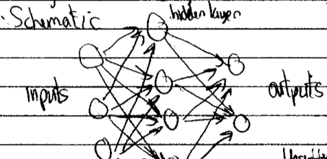
Train with a set of inputs and outputs (supervised learning), which determines the weights that dictate how inputs are mapped to outputs. Unsupervised learning has inputs and a cost function to be minimized.
This is a very versatile way to reproduce functions.
ML is used for classification (what numeral is that? what phase? cat or not?) and regression (learn a function).
Inputs \(x_1,\ldots, x_p\) depend on details of the problem.
One node:
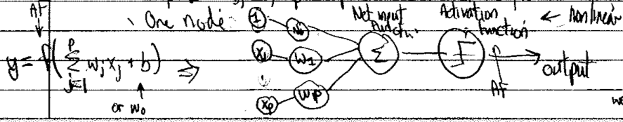
In the example one node would be one \(j\). Then \(U_{ij} \rightarrow W_i\), \(\tanh\) is the AF, and we only consider one output.