4.9. Lecture 12
Integration and marginalization by sampling: intuition
Integration
Comparison of integration methods
Approximation by Riemann sum (or trapezoid rule).
Approximation using MCMC samples.
Suppose we want to calculate the expectation value of a function \(f(x)\) where the distribution of \(x\) is \(p(x|D,I)\) and we’ll restrict the domain of \(x\) to the positive real axis. So
(4.7)¶\[ \langle f\rangle = \int_{0}^\infty f(x) p(x|D,I) dx \]and we’ll imagine \(p(x|D,I)\) is like the red lines in the figures here.
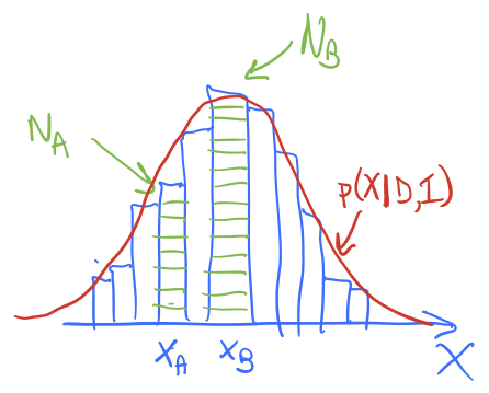
In method 1, we divide the \(x\) axis into bins of width \(\delta x\), let \(x_i = i\cdot\Delta x\), \(i=0,\ldots,N-1\). Then
\[ \langle f\rangle \approx \sum_{i=0}^{N-1} f(x_i)\, p(x_i|D,I) \,\Delta x . \]The histogram bar height tells us the strength of \(p(x_i|D,I)\) and we have a similar discretization for \(f(x)\).
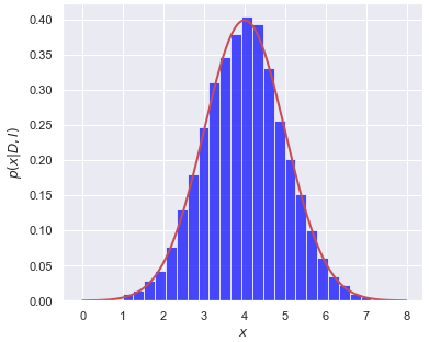
In method 2, we sample \(p(x|D,I)\) to obtain a representative set of \(x\) values, which we’ll denote by \(\{x_j\}\), \(j=0,\ldots,N'-1\). If I histogram \(\{x_j\}\) it looks like the posterior, as seen in the figures. To approximate the expectation value, we simply use:
\[ \langle f\rangle \approx \frac{1}{N'}\sum_{j=0}^{N'-1} f(x_j) . \]In method 1, the function \(p(x | D,I)\) weights \(f(x)\) at \(x_i\) by multiplying by the value of \(p(x_i|D,I\)), so strong weighting near the peak of \(p\) and weak weighting far away. The amount of the weighting is given (approximately) by the height of the corresponding histogram bar. In method 2, we have similar weighting of \(f(x)\) near to and far from the peak of \(p\), but instead of this being accomplished by multiplying by \(p(x_j|D,I)\), there are more \(x_j\) values near the peak than far away, in proportion to \(p(x_j|D,I)\). In the end it is the same weight!
Marginalization
Return to the expectation value of \(x\) in Eq. (4.7), but now suppose we introduce a nuisance parameter \(y\) into the distribution:
(4.8)¶\[ p(x|D,I) = \int_{0}^{\infty} dy\, p(x,y|D,I) \]And now we sample \(p(x,y|D,I)\) using MCMC to obtain samples \(\{(x_j,y_j)\}\), \(j=0,\ldots,N'-1\).
If we had a function of \(x\) and \(y\), say \(g(x,y)\), that we wanted to take the expectation value, we could use our samples as usual:
(4.9)¶\[ \langle g \rangle \approx \frac{1}{N'}\sum_{j=0}^{N'-1} g(x_j,y_j) . \]But suppose we just have \(f(x)\), so we want to integrate out the \(y\) dependence; e.g., going backwards in (4.8)? How do we do that with our samples \(\{(x_j,y_j)\}\)?
(4.10)¶\[\begin{split}\begin{align} \langle f \rangle &= \int_{0}^\infty dx f(x)\int_{0}^{\infty} dy\, p(x,y|D,I) \\ &\approx \frac{1}{N'}\sum_{j=0}^{N'-1} f(x_j) . \end{align}\end{split}\]Equivalently we can note that \(f(x)\) is just a special case of \(g(x,y)\) with no \(y\) dependence. Then (4.9) gives the same formula for \(\langle f\rangle\) as (4.10).
So to marginalize, we just use the \(x\) values in each \((x_j,y_j)\) pair. I.e., we ignore the \(y_j\) column!
MCMC Sampling Interlude: Assessing Convergence
We’ve seen that using MCMC with the Metropolis-Hastings algorithm can lead to a Markov chain: a set of confiurations of the parameters we are sampling. This chain enables inference because they are samples of the posterior of interest.
But how do we know the chain is converged? That is, that it is providing samples of the stationary distribution? We need diagnostics of convergence!
What can go wrong?
Could fail to have converged.
Could exhibit apparent convergence but the full posterior has not been sampled.
Convergence could be only approximate because the samples are correlated (need to run longer).
Strategies to monitor convergence:
Run multiple chains with distributed starting points.
Compute variation between and within chains \(\Lra\) look for mixing and stationarity.
Make sure the acceptance rate for MC steps is not too low or too high.
In this schematic version of Figure 11.3 in BDA-3, we see on the left two chains that stay in separate regions of \(\theta_0\) (no mixing) while on the right there is mixing but neither chain shows a stationary distribution (the \(\theta_0\) distribution keeps changing with MC steps).

Step through the MCMC-diagnostics.ipynb notebook, which goes through a laundry list of diagnostics. We’ll return to these later in the context of
pymc3.Some notes:
In BDA-3 Figure 11.1, a) is not converged; b) has 1000 iterations and is possibly converged; c) shows (correlated) draws from the target distribution.
We’re doing straight-line fitting again using the
emceesampling, but now with the Metropolis-Hasting algorithm (more below on the default algorithm).In
emcee, we usemoves.GaussianMove(cov), which implements a Metropolis step using a Gaussian proposal with mean zero and covariancecov.# MH-Sampler setup stepsize = .005 cov = stepsize * np.eye(ndim) p0 = np.random.rand(nwalkers,ndim) # initialize the sampler sampler = emcee.EnsembleSampler(nwalkers, ndim, log_posterior, args=[x, y, dy], moves=emcee.moves.GaussianMove(cov))
The covariance
covcould be a scalar, as it is here, or a vector or a matrix. See the relevant emcee manual page for further details and more general moves.The
stepsizeparameter is at our disposal to explore the consequences on convergence of it being too large or too small.To get the chains from the above code snippet we use
sampler.chain, which will give a list with the shape (# walkers, # steps, # dimensions). So 10 walkers taking 2000 steps each for a two-dimensional posterior (that is, \(\thetavec\) has two components) has the shape (10, 2000, 2). We can combine the results from all the walkers withsampler.chain.reshape((-1,ndim)), which flattens the first two axes of the list. (One reshape dimension can always be \(-1\), which infers the value from the length of the array. So here the reshaped array will have two axes with the second one having dimensionndim.)How do we know a chain has converged to a representation of the posterior? Standard error of the mean \(SE(\overline\thetavec)\).
This asks how the mean of \(\thetavec\) deviates in the chain from the true distribution mean. Thus it is the simulation (or sampling) error of the mean, not the underlying uncertainty ( or spread) of \(\thetavec\).
Calculate it for \(N\) samples as
\[ SE(\overline\thetavec) = \frac{\text{posterior standard deviation}}{\sqrt{N}} \]Visualize this with a moving average \(\Lra\) check for stability.
Autocorrelation: do you recognize the formula in the code?
Acceptance rate. Usually autotuned in packaged MCMC software.
Assess the mixing with the Gelman-Rubin diagnostic.
We’ll come back to this later, so this is just a quick pass.
Basic idea: multiple chains from different walkers (after warm-up) are split up and one looks at the variance within a chain and between chain.
There is some internal documentation in the notebook; see BDA-3 pages 284-5 for more details.
Try changing the
step_sizein the notebook to see what happens to each of the diagnostics.Point of emphasis: “The key purpose of MCMC is not to explore the posterior but to estimate expectation values.”
Figures to make every time you run MCMC (following Hogg and Foreman-Mackey sect. 9)
Trace plots
The burn-in length can be seen; can identify problems with model or sampler; qualitative judge of convergence.
Use convergence diagnostic such as Gelman-Rubin.
Corner plots
If you have a \(D\)-dimensional parameter space, plot all \(D\) diagonal and all \({D\choose 2}\) joint histograms to show low-level covariances and non-linearities.
“… they are remarkable for locating expected and unexpected parameter relationships, and often invaluable for suggesting re-parameterizations and transformation that simplify your problem.”
Posterior predictive plots
Take \(K\) random samples from your chain, plot the prediction each sample makes for the data and over-plot the observed data.
“This plot gives a qualitative sense of how well the model fits the data and it can identify problems with sampling or convergence.”