1.8. Lecture 3
Step through the medical example key
Some of the answers are straightforward but make sure you agree with your neighbors. We’ll split out a few follow-up points.
Follow-up question on 2.
Why is it \(p(H|D)\) and not \(p(H,D)\)?
Answer
Recall that \(p(H,D) = p(H|D) \cdot p(D)\). You are generally interested in \(p(H|D)\). If you know \(p(D) = 1\), then they are the same.
Follow-up question on 5.
The emphasis here is on the sum rule. Why didn’t any column except Total in the sum/product rule notebook add to 1?
Answer
Because were were looking at \(p(\text{tall,blue}) + p(\text{short,blue}) \neq 1\), whereas \(p(\text{tall}| \text{blue}) + p(\text{short}| \text{blue}) = 1\).
In general and for 6. in particular we emphasise the usefulness of Bayes’ theorem to express \(p(H|D)\) in terms of \(p(D|H)\).
Make sure that 8. and 9. are clear to you. In 8., this is standard but not so obvious at first; after it becomes familiar you will find that you jump right to the end.
Recap of coin flipping notebook
Recall the names of the pdfs in Bayes’ theoem: posterior, likelihood, prior, evidence; and recall Bayesian updating: prior + data \(\rightarrow\) posterior \(\rightarrow\) updated prior \(\rightarrow\) updated posterior \(\rightarrow\) \(\ldots\).
Take-aways and follow-up questions from coin flipping:
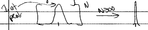
Different priors eventually give the same posterior with enough data. This is called Bayesian convergence. How many tosses are enough? Hit
New Datamultiple times to see the fluctuations. Clearly it depends on \(p_h\) and how close you want the posteriors to be. How about for \(p_h = 0.4\) or \(p_h = 0.9\)?Answer
\(p_h = 0.4\) \(\Longrightarrow\) \(\approx 200\) tosses will get you most of the way.
\(p_h = 0.9\) \(\Longrightarrow\) much longer for the informative prior than the others.
Why does the “anti-prior” work well even though its dominant assumptions (most likely \(p_h = 0\) or \(1\)) are proven wrong early on?
Answer
The “heavy tails” (which in general means the probability away from the peaks; in the middle for the “anti-prior”) mean it is like uniform (renormalized!) after the ends are eliminated. An important lesson for formulating priors: allow for deviations from your expectations.
Case I and Case II for priors both use the beta distribution as a conjugate prior (the uniform case is included as \(\alpha=1,\beta=1\)). From the code for updating:
y_i = stats.beta.pdf(x,alpha_i + heads, beta_i + N - heads)Is there a difference between updating sequentially or all at once? Do the simplest problem first: two tosses. Let results be \(D = \{D_k\}\) (in practice take 0’s and 1’s as the two choices \(\Longrightarrow\) \(R = \sum_k D_k\)).
The general relation is \(p(p_h | \{D_k\},I) \propto p(\{D_k\}|p_h,I) p(p_h|I)\) by Bayes’ theorem.
First \(k=1\) (so \(D_1 = 0\) or \(D_1 = 1\)):
(1.13)¶\[ p(p_h | D_1,I) \propto p(D_1|p_h,I) p(p_h|I)\]Now \(k=2\), starting with the expression for updating all at once and then using the sum and product rules (including their corollaries marginalization and Bayes’ Rule) to move the \(D_1\) result to the right of the \(|\) so it can be related to sequential updating:
(1.14)¶\[\begin{split}\begin{align} p(p_h|D_2, D_1) &\propto p(D_2, D_1|p_h, I)\times p(p_h|I) \\ &\propto p(D_2|p_h,D_1,I)\times p(D_1|p_h, I)\times p(p_h|I) \\ &\propto p(D_2|p_h,D_1,I)\times p(p_h|D_1,I) \\ &\propto p(D_2|p_h,I)\times p(p_h|D_1,I) \\ &\propto p(D_2|p_h,I)\times p(D_1|p_h,I) \times p(p_h,I) \end{align}\end{split}\]What is the justification for each step?
1st line: Bayes’ Rule
2nd line: Product Rule (applied to \(D_1\))
3rd line: Bayes’ Rule (going backwards)
4th line: tosses are independent
5th line: Bayes’ Rule on the last term in the 3rd line
The fourth line of (1.14) is the sequential result! (The prior for the 2nd flip is the posterior (1.13) from the first flip.)
So all at once is the same as sequential as a function of \(p_h\), when normalized!
To go to \(k=3\):
\[\begin{split}\begin{align} p(p_h|D_3,D_2,D_1,I) &\propto p(D_3|p_h,I) p(p_h|D_2,D_1,I) \\ &\propto p(D_3|p_h,I) p(D_2|p_h,I) p(D_1|p_h,I) p(p_h) \end{align}\end{split}\]and so on.
What about “bootstrapping”? Why can’t we use the data to improve the prior and apply it (repeatedly) for the same data. I.e., use the posterior from the first set of data as the prior for the same set of data. Let’s see what this leads to (we’ll label the sequence of posteriors we get \(p_1,p_2,\ldots,p_N\)):
\[\begin{split}\begin{align} p_1(p_h | D_1,I) &\propto p(D_1 | p_h, I) \, p(p_h | I) \\ \\ \Longrightarrow p_2(p_h, D_1, I) &\propto p(D_1 | p_h, I) \, p_1(p_h | D_1, I) \\ &\propto [p(D_1 | p_h,I)]^2 \, p(p_h | I) \\ \mbox{keep going?}\quad & \\ p_N(p_h | D_1, I) &\propto p(D_1|p_h, I)\, p_{N-1}(p_h | D_1, I) \\ &\propto [p(D_1 | p_h, I)]^N \, p(p_h | I) \end{align}\end{split}\]Suppose \(D_1\) was 0, then \([p(\text{tails}|p_h,I)]^N \propto (1-p_h)^N p(p_h|I) \overset{N\rightarrow\infty}{\longrightarrow} \delta(p_h)\) (i.e., the posterior is only at \(p_h=0\)!). Similarly, if \(D_1\) was 1, then \([p(\text{tails}|p_h,I)]^N \propto p_h^N p(p_h|I) \overset{N\rightarrow\infty}{\longrightarrow} \delta(1-p_h)\) (i.e., the posterior is only at \(p_h=1\).)
More generally, this bootstrapping procedure would cause the posterior to get narrower and narrower with each iteration so you think you are getting more and more certain, with no new data!
Warning
Don’t do that!
Something to come back to: Frequentist point estimates
Maximum-likelihood means: what value of \(p_h\) maximizes the likelihood (notation: \(\mathcal{L}\) is often used for the likelihood)
Answer
Similarly, the standard deviation is \(\sigma = \sqrt{p_h(1-p_h)/N}\).
Different types of independence (see question 5. in radioactive-lighthouse notebook)
Let’s suppose we flip two fair coins. Consider the propositions:
\(A\): 1st coin comes up heads
\(B\): 2nd coin comes up heads
\(C\): the two results are the same
\(A\) and \(B\) are independent: \(p(A,B) = p(A|B)p(B) = p(A) p(B)\) and each is equal to 1/2.
\(A\), \(B\), and \(C\) are pairwise independent:
\(\Lra\) we don’t know anything more given the proposition to the right of the \(|\).
But \(A\) and \(B\) are not conditionally independent given \(C\). In particular, if you know \(A\) and \(C\) are true, then \(B\) is determined! In the radioactive lighthouse case, knowing \(x_0,y_0\) tells us about \(x_2\), but also knowing \(x_1\) tells us nothing in addition.