2.12. Follow-up: fluctuation trends with # of points and data errors
This is a follow-up to Assignment: Follow-ups to Parameter Estimation notebooks, which focuses on the trends of fluctuations and how to visualize them.
A. Parameter estimation example: fitting a straight line
2. Do exercise 3: “Change the random number seed to get different results and comment on how the maximum likelihood results fluctuate. How are size of the fluctuations related to the number of data points \(N\) and the data error standard deviation \(dy\)? (Try changing them!)”
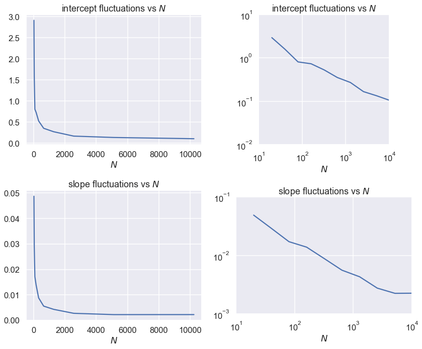
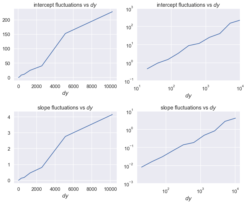
The size of the fluctuations decrease as the square root of the number of points N. As the data error standard deviation increases, the size of the fluctuations increases linearly with dy.
How do we obtain, visualize, and understand these results?
%matplotlib inline
import matplotlib.pyplot as plt
import numpy as np
import seaborn; seaborn.set('talk') # for plot formatting
from scipy import optimize

def make_data(intercept, slope, N=20, dy=5, rseed=None):
    """Given a straight line defined by intercept and slope:
          y = slope * x + intercept
       generate N points randomly spaced points from x=0 to x=100
       with Gaussian (i.e., normal) error with mean zero and standard
       deviation dy.

       Return the x and y arrays and an array of standard deviations.
    """
    rand = np.random.RandomState(rseed)
    x = 100 * rand.rand(N)  # choose the x values randomly in [0,100]
    y = intercept + slope * x  # This is the y value without noise
    y += dy * rand.randn(N)    # Add in Gaussian noise
    return x, y, dy * np.ones_like(x)  # return coordinates and error bars

def log_likelihood(theta, x, y, dy):
    y_model = theta[0] + theta[1]*x
    return -0.5*np.sum(np.log(2*np.pi*dy**2)+ (y - y_model)**2/dy**2)

def minfunc(theta, x, y, dy):
    """
    Function to be minimized: minus the logarithm of the likelihood.
    """
    return -log_likelihood(theta, x, y, dy)
First make tables
intercept = 25.   # true intercept (called b elsewhere)
slope = 0.5       # true slope (called m elsewhere)
theta_true = [intercept, slope]  # put parameters in a true theta vector

iterations = 10
# Fix dy and vary Npts geometrically
dy_data = 5
for Npts in [20, 80, 320]:
    print(f'N = {Npts}, dy = {dy_data}')
    print('          intercept   slope')
    print(f'true:       {intercept:.3f}    {slope:.3f}')

    for i in np.arange(iterations):
        x, y, dy = make_data(*theta_true, N=Npts, dy=dy_data, rseed=None)
        result = optimize.minimize(minfunc, x0=[0, 0], args=(x, y, dy))
        intercept_fit, slope_fit = result.x

        print(f'dataset {i}:  {intercept_fit:.3f}    {slope_fit:.3f}')
    print('------------------------------\n')
N = 20, dy = 5
          intercept   slope
true:       25.000    0.500
dataset 0:  26.121    0.488
dataset 1:  24.379    0.477
dataset 2:  28.448    0.406
dataset 3:  31.338    0.434
dataset 4:  19.791    0.566
dataset 5:  23.434    0.500
dataset 6:  21.570    0.543
dataset 7:  23.114    0.549
dataset 8:  28.597    0.457
dataset 9:  19.860    0.545
------------------------------

N = 80, dy = 5
          intercept   slope
true:       25.000    0.500
dataset 0:  24.694    0.508
dataset 1:  25.215    0.490
dataset 2:  24.527    0.520
dataset 3:  24.962    0.485
dataset 4:  23.997    0.499
dataset 5:  24.504    0.497
dataset 6:  23.002    0.529
dataset 7:  22.897    0.537
dataset 8:  24.026    0.514
dataset 9:  24.027    0.502
------------------------------

N = 320, dy = 5
          intercept   slope
true:       25.000    0.500
dataset 0:  25.780    0.496
dataset 1:  24.403    0.505
dataset 2:  25.067    0.504
dataset 3:  24.019    0.518
dataset 4:  25.243    0.498
dataset 5:  24.903    0.494
dataset 6:  25.476    0.497
dataset 7:  24.273    0.508
dataset 8:  25.363    0.496
dataset 9:  24.602    0.499
------------------------------
# Fix Npts and vary dy geometically
Npts = 80
for dy_data in [1, 5, 25]:
    print(f'N = {Npts}, dy = {dy_data}')
    print('          intercept   slope')
    print(f'true:       {intercept:.3f}    {slope:.3f}')

    for i in np.arange(iterations):
        x, y, dy = make_data(*theta_true, N=Npts, dy=dy_data, rseed=None)
        result = optimize.minimize(minfunc, x0=[0, 0], args=(x, y, dy))
        intercept_fit, slope_fit = result.x

        print(f'dataset {i}:  {intercept_fit:.3f}    {slope_fit:.3f}')
    print('------------------------------\n')
N = 80, dy = 1
          intercept   slope
true:       25.000    0.500
dataset 0:  25.281    0.494
dataset 1:  24.989    0.504
dataset 2:  25.134    0.499
dataset 3:  25.022    0.502
dataset 4:  24.651    0.512
dataset 5:  25.229    0.497
dataset 6:  24.828    0.502
dataset 7:  25.318    0.495
dataset 8:  25.282    0.497
dataset 9:  25.282    0.495
------------------------------

N = 80, dy = 5
          intercept   slope
true:       25.000    0.500
dataset 0:  24.720    0.508
dataset 1:  23.637    0.521
dataset 2:  26.342    0.468
dataset 3:  24.035    0.514
dataset 4:  26.363    0.462
dataset 5:  23.992    0.523
dataset 6:  25.620    0.485
dataset 7:  25.440    0.502
dataset 8:  25.571    0.475
dataset 9:  26.452    0.472
------------------------------

N = 80, dy = 25
          intercept   slope
true:       25.000    0.500
dataset 0:  20.129    0.527
dataset 1:  18.857    0.604
dataset 2:  18.320    0.707
dataset 3:  27.873    0.399
dataset 4:  19.448    0.561
dataset 5:  21.213    0.558
dataset 6:  19.209    0.550
dataset 7:  16.658    0.656
dataset 8:  28.626    0.451
dataset 9:  24.319    0.450
------------------------------
Now make a function for rerunning
def std_of_fit_data(Npts, dy_data, iterations, theta_true=theta_true):
    """Calculate the standard deviations of the slope and intercept
       for a given number of iterations
    """
    intercept_fits = np.zeros(iterations)
    slope_fits = np.zeros(iterations)

    for j in np.arange(iterations):
        x, y, dy = make_data(*theta_true, N=Npts, dy=dy_data, rseed=None)
        result = optimize.minimize(minfunc, x0=[0, 0], args=(x, y, dy))
        intercept_fits[j], slope_fits[j] = result.x

    return intercept_fits.std(), slope_fits.std()
std_of_fit_data(20, 5, 20)
(3.3694189754675885, 0.05485217437350401)
std_of_fit_data(80, 5, 20)
(1.1785970628509084, 0.018145922809239247)
std_of_fit_data(320, 5, 20)
(0.5223960837377885, 0.008440770742473696)
Now make linear and log-log plots
Which is better? How do you read a power law from a log-log plot?
Npts_array = [20 * 2**i for i in range(10)]
Npts_array
[20, 40, 80, 160, 320, 640, 1280, 2560, 5120, 10240]
# Fix dy and vary Npts geometrically
dy_data = 5

Npts_array = [20 * 2**j for j in range(10)]
intercept_std_array = np.zeros(len(Npts_array))
slope_std_array = np.zeros(len(Npts_array))

iterations = 20
for i, Npts in enumerate(Npts_array):
    intercept_std_array[i], slope_std_array[i] = std_of_fit_data(Npts, dy_data, iterations)

fig, axes = plt.subplots(2, 2, figsize=(12, 10))

axes[0,0].set_title(r'intercept fluctuations vs $N$')
axes[0,0].set_xlabel(r'$N$')
axes[0,0].plot(Npts_array, intercept_std_array)

axes[0,1].set_title(r'intercept fluctuations vs $N$')
axes[0,1].set_xlabel(r'$N$')
axes[0,1].loglog(Npts_array, intercept_std_array)
axes[0,1].set_xlim(10,1e4)
axes[0,1].set_ylim(.01,10)
axes[0,1].set_aspect('equal')

axes[1,0].set_title('slope fluctuations vs $N$')
axes[1,0].set_xlabel(r'$N$')
axes[1,0].plot(Npts_array, slope_std_array)

axes[1,1].set_title('slope fluctuations vs $N$')
axes[1,1].set_xlabel(r'$N$')
axes[1,1].loglog(Npts_array, slope_std_array)
axes[1,1].set_xlim(10,1e4)
axes[1,1].set_ylim(1e-3,1e-1)
axes[1,1].set_aspect('equal')

fig.tight_layout()
# Fix Npts and vary dy geometrically
Npts = 20

dy_array = [1 * 2**j for j in range(10)]
intercept_std_array = np.zeros(len(dy_array))
slope_std_array = np.zeros(len(dy_array))

iterations = 20
for i, dy_data in enumerate(dy_array):
    intercept_std_array[i], slope_std_array[i] = std_of_fit_data(Npts, dy_data, iterations)

fig, axes = plt.subplots(2, 2, figsize=(12, 10))

axes[0,0].set_title(r'intercept fluctuations vs $dy$')
axes[0,0].set_xlabel(r'$dy$')
axes[0,0].plot(Npts_array, intercept_std_array)

axes[0,1].set_title(r'intercept fluctuations vs $dy$')
axes[0,1].set_xlabel(r'$dy$')
axes[0,1].loglog(Npts_array, intercept_std_array)
axes[0,1].set_xlim(1e1,1e4)
axes[0,1].set_ylim(.1,1000)
#axes[0,1].set_aspect('equal')

axes[1,0].set_title('slope fluctuations vs $dy$')
axes[1,0].set_xlabel(r'$dy$')
axes[1,0].plot(Npts_array, slope_std_array)

axes[1,1].set_title('slope fluctuations vs $dy$')
axes[1,1].set_xlabel(r'$dy$')
axes[1,1].loglog(Npts_array, slope_std_array)
axes[0,1].set_xlim(1e1,1e4)
axes[1,1].set_ylim(1e-3,1e+1)
#axes[1,1].set_aspect('equal')

fig.tight_layout()
In both sets of joint posterior graphs, are the slope and intercept correlated? How do you know? Does it make sense?
For the first set of data, answer the question: “What do you conclude about how the form of the prior affects the final posterior in this case?”
For the second set of data, answer the question: “Why in this case does the form of the prior have a clear effect?” You should consider both the size of the error bars and the number of data points (try changing them to explore the impact).