5.4. Lecture 16
Computational possibilities for evidence
Many possible challenges:
Likelihood sharply peaked in prior range, but could have long tails and significant contribution to integrals.
Likelihood could be multimodal.
Posterior may only be significant on thin “sheets” in parameter space (cf. sampling visualization).
Trotta summary of methods: (possibly out-of-date in places)
Thermodynamic integration \(\longrightarrow\) simulated anneling.
Computational cost depends heavily on dimensionalisty of parameter space and on details of likelihood function.
Cosmological applications require up to \(10^7\) likelihood evaluations (100 times MCMC-based parameter estimation).
Parallel tempering (more to follow!).
Nested sampling recasts multidimensional evidence integral into one-dimensional integral, which is easy to evaluate numerically.
Takes \(\sim 10^5\) likelihood evaluations.
multinest is more efficient still.
Approximations to the Bayes factor:
If models are nested: ask whether new parameter is supported by data.
Laplace approximation may be good but be careful of priors.
Define the effective number of parameters (see BDA3)
AIC, BIC, DIC, WAIC (summary to follow; see BDA3 for details)
The paper “Practical Bayesian model evaluation using leave-one-out cross-validation and WAIC” by Vehtari, Gelman, and Gabry is a good (and reliable) source for theoretical and practical details on assessing and comparing the predictive accuracy of different models. Quote: “Cross-validation and information criteria are two approaches to estimating out-of-sample predictive accuracy using within-sample fits.” The computations use the log-likelihood evaluated at posterior simulations of the parameters.
Examples of information criteria
These are computationally much easier than full evaluations of the evidence.
AIC: Akaiko Information Criteria
Essentially frequentist as it relies solely on the likelihoo
Quantity to calculate:
\[ \textit{AIC} = -2 \log p(D|\hat\thetavec_{\text{MLE}}) + 2k \]where \(k\) is the number of free parameters and the probability distribution is the likelihood evaluated at the maximum likelihood values of the parameters.
Compare the resulting quantity between the models.
Has the ingredients of evidence: improved likelihood is balanced by a penalty for additional parameters. No priors.
Not well regarded by Bayesians.
BIC: Bayesian Information Criteria
Gaussian approximation to Bayesian evidence in limit of large amount of data.
\[ \textit{BIC} = -2 \log p(D|\hat\thetavec_{\text{MLE}}) + k\ln N \]where \(k\) is the number of fitted parameters and \(N\) is the number of data points.
Assumes that the Occam penalty is negligible.
DIC: Deviance Information Criteria
Replace \(\hat\thetavec_{\text{MLE}}\) by \(\hat\thetavec_{\text{Bayes}}\), where the latter is the maximum of the posterior (as opposed to the maximum of the likelihood).
Use the effective number of parameters:
\[ p_{DIC} = 2\log p(D|\hat\thetavec_{\text{Bayes}}) - E[\log p(D|\thetavec)] \]where the last term averages \(\thetavec\) over the posterior.
Then
\[ \textit{DIC} = -2 \log p(D|\hat\thetavec_{\text{Bayes}}) + 2 p_{DIC} . \]
WAIC: Widely Applicable Information Criteria*
Favored by BDA-3 as more fully Bayesian
Given samples \(s = 1\) to \(S\):
\[ \textit{WAIC} = 2\sum_{i=1}^{n_{\text{data}}} \Bigl(\log \frac{1}{S}\sum_{s=1}^S p(y_i|\thetavec^s)\Bigr) - \frac{1}{S}\sum_{s=1}^S \log p(D_i|\thetavec^s) \]Averages over the posterior distribution.
Application of Information Criteria and Bayes factors
An example of applying Bayesian methods to perform model comparisons is “Model comparison tests of modified gravity from the Eöt-Wash experiment” by Krishak and Desai. They re-examine the claim in “Hints of Modified Gravity in Cosmos and in the Lab?”” by Perivolaropoulos and Kazantzidis, made using frequentist methods, that there is evidence in the data of the Eöt-Wash experiment that looks for modifications of Newton’s Law of Gravity on sub-millimeter scales for a residual spatially oscillating signal in the data. This could point to a modification of general relativity (in particular, of some type of nonlocal gravity theory) or it could be due to statistical or systematic uncertainties in the data.
The experiment under consideration is a modern version of the classic torsion balance experiments to measure the force due to gravity. In particular, it is sensitive to departures from Newtonian gravity at sub-millimeter scales. The data analysis from the experimenters do not indicate signs of new physics, but the re-analysis by Perivolaropoulos and Kazantzidis claims that the residual data has signatures of an oscillating signal.
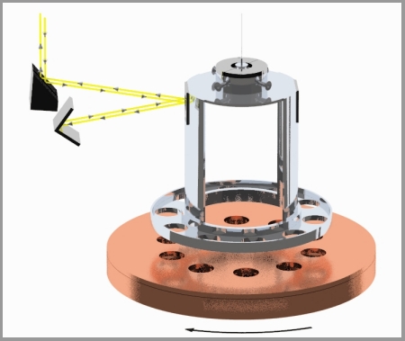
From https://www.npl.washington.edu/eotwash/inverse-square-law: “Below is a cartoon of one of our initial experimental devices which illustrates the technique we employ to measure gravity at short length scales. The pendulum ring, with 10 small holes bored into it, hangs by a thin tungsten fiber (typically 20 microns thick) and acts as the detector mass. The rotating plate just below it, with 10 similar holes bored into it, acts as the drive mass providing gravitational pull on the pendulum that twists it back and forth 10 times for every revolution of the plate. The pendulum twist is measured by shining a laser beam off of a mirror mounted above the ring. The induced twist (torque) on the pendulum at varying separation distances is then compared to a detailed Newtonian calculation of the system. For many of our measurements, the rotating attractor situated just below the detector ring actually consists of 2 disks. The upper disk has holes identical to those in the detector ring. The lower, thicker attractor disk also has a similar hole pattern bored into it, but these larger holes are rotated compared to those in the upper disk, so that they lie halfway between the holes in the upper disk. If the inverse-square law is correct, the lower holes are designed such that they produce a twist on the ring that just cancels the twist induced by the upper disk. However, if gravity changes strength at short distances as the theories suggest, the twist induced by the lower disk, which is farther from the ring, will no longer cancel the twist from the upper disk and we will see a clear twist signal. The actual situation is a bit more complicated; for ordinary gravity the cancellation is exact only for one particular separation between the ring and the attractor, but the variation of the magnitude of the twist with changing separation between the ring and the disks provides a clear ‘signature’ for any new gravitational or other short-range phenomena.”
There are 87 residual torque data points (\(\delta \tau\)) between measured torques and expected Newtonian values. Perivolaropoulos and Kazantzidis made fits to three functions (models):
\[\begin{split}\begin{align} \delta\tau_1(\alpha',m',r) &= \alpha' \qquad \text{offset Newtonian potential} \\ \delta\tau_2(\alpha',m',r) &= \alpha' e^{-m'r} \\ \delta\tau_3(\alpha',m',r) &= \alpha' \cos(m'r + \phi) \end{align}\end{split}\]Figures of the data and some fits from figures in the two papers are shown here.


Next we have tables from Krishak and Desai showing the best-fit results and the adopted priors.
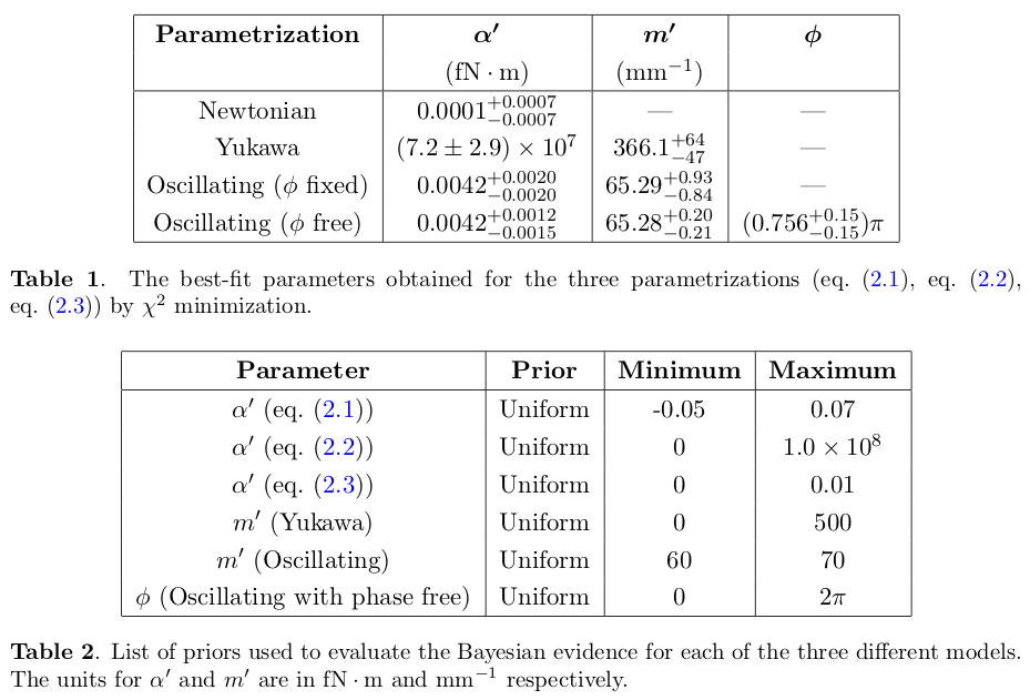
Krishak and Desai applied AIC, BIC, WAIC, and calculated the Bayes factor (ratio of Bayesian evidences).
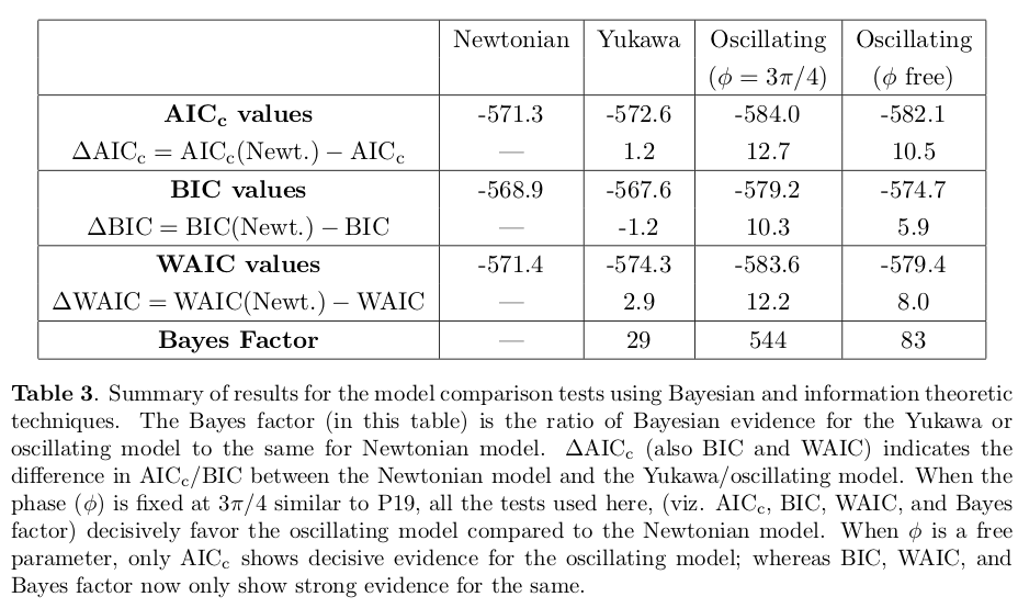
Conclusions were based on interpretive scales found in the literature. For example:
\(\Delta\)BIC
Evidence against Model \(i\)
0 − 2
Not Worth More Than A Bare Mention
2 − 6
Positive
6 − 10
Strong
\(> 10\)
Very Strong
For interpreting the Bayes’ factor the Jeffrey’s scale is used: a value above 10 represents strong evidence in favor of the model in the numerator while a value above 100 represents decisive evidence.
Krishak and Desai conclude that there is decisive support that the oscillating model with fixed phase (from the Perivolaropoulos and Kazantzidis fit) and strong evidence for varying phase. However, this statistical analysis does not distinguish between a physics origin and statistical effects in the data.
Krishak and Desai use nested sampling software to evaluate the evidence.
Parallel tempering
Parallel tempering was particularly introduced to deal with multimodal distributions (see simulation for example).
Analogous to the problem of global (as opposed to local) optimization, which can mean either minimizing or maximizing a function.
Tricky: how do you jump from one region of high posterior density to another when there is a large region of low probability in between?
This is a problem for an evidence calculation, because we need to integrate over the entire parameter space.
For parameter estimation, it may be sufficient to start walkers in the vicinity of the “best” (highest posterior) part of the posterior.
Parallel tempering is built on top of an MCMC sampler.
The general idea is to simulate \(N\) replicas of a system, each at a different temperature.
The temperature of a Metropolis-Hastings Markov chain specifies how likely it is to sample from a low-density part of the target distribution.
At high temperature, large volumes of phase space are sampled roughly, while low temperature systems have precise sampling in a local region of the parameter space, where they can get stuck in a local energy minimum (meaning a local posterior maximum).
Parallel tempering works by letting the systems at different temperatures exchange configurations, which enables the low \(T\) system access to a complete set of low-temperature regions.
The temperature comes in analogy to a Boltzmann factor \(e^{-E/k_B T}= e^{-\beta E}\) where \(\beta \equiv 1/k_B T\).
Instead of \(E\) we have \(-\log p_\beta(x)\) so
\[ p_\beta(x) = e^{-\beta(-\log p(x))} = \bigl(p(x)\bigr)^\beta \]We seek the posterior written with Bayes’ theorem and normalization constant \(C\):
\[ p(\thetavec|D,I) = C p(D|\thetavec,I) p(\thetavec|I) \]and generalize to the temperature-dependent posterior \(p_\beta\):
\[ p_{\beta(\thetavec|D,I)} \propto p(D|\thetavec,I)^\beta p(\thetavec|I) \qquad 0 \leq \beta \leq 1 \]or
\[ \log p_{\beta(\thetavec|D,I)} = C + \beta\log p(D|\thetavec,I) + \log p(\thetavec|I) . \]So the desired distribution is \(\beta = 1\), and \(\beta = 0\) is the prior alone.
At large temperature, \(\beta = 0\), and we sample the prior, which should encompass the full (accessible) space.
As we approach \(\beta = 1\) we fous increasingly on where the likelihood is large.
We will use \(\beta \in \{1,\beta_2, \ldots, \beta_N\}\) running in parallel, but swapping members of the chains in such a way that detailed balance is preserved.
The general sampling strategy is:
at intervals, pick a pair of adjacent chains at random: \(\beta_i\) and \(\beta_{i+1}\);
propose a swap of their current positions at this time \(t\), namely exchange \(\thetavec_{t,i}\) and \(\thetavec_{t,i+1}\);
accept this proposal with probability (note the \(i\)s and \((i+1)\)s):
\[ r = \min\left\{1, \frac{p_\beta(\thetavec_{t,i+1}|D,\beta_i,I) p_\beta(\thetavec_{t,i}|D,\beta_{i+1},I)} {p_\beta(\thetavec_{t,i}|D,\beta_i,I) p_\beta(\thetavec_{t,i+1}|D,\beta_{i+1},I)} \right\} \]This will preserve detailed balance.
We can make this expression more intuitive if we connect back to the physics analogy.
\[ p_\beta(\thetavec|D,I) \propto p(D|\thetavec,I)^\beta p(\thetavec|I) \propto e^{-\beta(-\log p(D|\thetavec,I)) p(\thetavec|I)} \]and \(-\log p(D|\thetavec,I)\) is the potential energy \(U(\rvec)\) (by analogy). Then the priors drop out of the ratio in \(r\) (the prior is independent of \(\beta\)), leaving:
\[ r = \min\left\{1,e^{-(\beta_i - \beta_{i+1})(U(\rvec_{i+1}-U(\rvec_i)))}\right\} \]so the four terms in \(r\) arise from the Boltzman factors of the energy difference at the two temperatures.
Things to specify for the sampler:
\(n_s\): propose a swap every \(n_s\) iterations, which is implemented by drawing a random number \(U_1 \sim \text{Uniform}[0,1]\) every iteration and proposing a swap if \(U_1 \leq 1/n_s\).
The length and spacing of the temperature ladder.
Calculating the evidence
To calculate the evidence from parallel tempering, we can use thermodynamic integration see Goggans and Chi, AIP Conf. Proc. 707, 59 (2004).
Define the temperature dependent evidence:
\[ Z(\beta) \equiv \int d\thetavec\, p(D|\thetavec,I)^\beta p(\thetavec|I) = \int d\thetavec\, e^{\beta\log p(D|\thetavec,I)} p(\thetavec|I) \]so we want \(Z(1)\).
\(Z(\beta)\) satisfies a differential equation:
\[\begin{split}\begin{align} \frac{d\log Z(\beta)}{d\beta} &= \frac{1}{Z(\beta)} \int d\thetavec \bigl(\log p(D|\thetavec,I)\bigr) p(D|\thetavec,I)^\beta p(\thetavec|I) \\ &\equiv \langle \log p(D|\thetavec,I\rangle_\beta , \end{align}\end{split}\]which is the average of the log likelihood at temperature \(\beta\).
So we can integrate over \(\beta\) (the first term is doesn’t contribute if the prior is normalized):
\[ \log Z(1) = \log Z(0) + \int_0^1 d\beta\, \langle \log p(D|\thetavec,I)\rangle_\beta , \]\(\Lra\) estimate from emcee samples by computing the average of \(p(D|\thetavec,I)\) within each chain and then evaluating the integral from a quadrature formula (e.g., Simpson’s rule).
Example of parallel tempering
An example of parallel tempering is given in MCMC-parallel-tempering_ptemcee.ipynb.
Comments:
First we set up a bi-modal distribution (it was originally intended to be a surprise, so the code was hidden). Just two Gaussians with different amplitudes.
A first sampling try with an ordinary Metropolis-Hastings (MH) sampler fails by only finding one mode.
But then if one checks two chains, separate modes are found but the chains do not mix. With many walkers one might find multiple modes, but the relative normalizations would not work because each walker would not explore the space.
The setup for
ptemceeincludes a temperature grid chosen so that numerically integrating over temperature for the evidence has a finer grid at low temperatures for greater accuracy.Note the corner plots for different temperatures and how the multimodal structure emerges.