Taylor problem 7.42
Taylor problem 7.42#
Last revised 25-Feb-2019 by Dick Furnstahl (furnstahl.1@osu.edu).
%matplotlib inline
import numpy as np
from scipy.integrate import solve_ivp

import matplotlib.pyplot as plt
# Change the common font size
font_size = 14
plt.rcParams.update({'font.size': font_size})
class Oscillator():
    """
    Oscillator class implements the parameters and differential equation for
     problem 7.42 from Taylor.

    Parameters
    ----------
    omega : float
        natural frequency of the pendulum (\sqrt{g/l} where l is the
        pendulum length)
    g : float
        acceleration due to gravity
    R : float
        radius parameter

    Methods
    -------
    dy_dt(t, y)
        Returns the right side of the differential equation in vector y,
        given time t and the corresponding value of y.
    solve_ode(t_pts, theta_0, theta_dot_0)
        Solves the ODE at t_pts given initial conditions.
    small_angle(t, epsilon)
        Returns the small angle solution.
    """
    def __init__(self, omega=np.sqrt(2.), g=1., R=1.):
        self.omega = omega
        self.g = g
        self.R = R
        self.theta_equil = np.arccos(self.g/(self.omega**2 * self.R))

    def dy_dt(self, t, y):
        """
        This function returns the right-hand side of the diffeq:
        [dtheta/dt d^2theta/dt^2]

        Parameters
        ----------
        t : float
            time
        y : float
            A 2-component vector with y[0] = theta(t) and y[1] = dtheta/dt

        Returns
        -------

        """
        return [y[1], (self.omega**2 * np.cos(y[0]) - self.g/self.R) \
                       * np.sin(y[0]) ]


    def solve_ode(self, t_pts, theta_0, theta_dot_0,
                  abserr=1.0e-10, relerr=1.0e-10):
        """
        Solve the ODE given initial conditions.
        For now use odeint, but we have the option to switch.
        Specify smaller abserr and relerr to get more precision.
        """
        y = [theta_0, theta_dot_0]
        solution = solve_ivp(self.dy_dt, (t_pts[0], t_pts[-1]),
                             y, t_eval=t_pts,
                             atol=abserr, rtol=relerr)
        theta, theta_dot = solution.y
        return theta, theta_dot

    def small_angle(self, t, epsilon_0):
        """Small angle solution"""
        Omega_prime = np.sqrt(self.omega**2 - (self.g/(self.omega*self.R))**2)
        return self.theta_equil + epsilon_0 * np.cos(Omega_prime * t)
def plot_y_vs_x(x, y, axis_labels=None, label=None, title=None,
                color=None, linestyle=None, semilogy=False, loglog=False,
                ax=None):
    """
    Generic plotting function: return a figure axis with a plot of y vs. x,
    with line color and style, title, axis labels, and line label
    """
    if ax is None:        # if the axis object doesn't exist, make one
        ax = plt.gca()

    if (semilogy):
        line, = ax.semilogy(x, y, label=label,
                            color=color, linestyle=linestyle)
    elif (loglog):
        line, = ax.loglog(x, y, label=label,
                          color=color, linestyle=linestyle)
    else:
        line, = ax.plot(x, y, label=label,
                    color=color, linestyle=linestyle)

    if label is not None:    # if a label if passed, show the legend
        ax.legend()
    if title is not None:    # set a title if one if passed
        ax.set_title(title)
    if axis_labels is not None:  # set x-axis and y-axis labels if passed
        ax.set_xlabel(axis_labels[0])
        ax.set_ylabel(axis_labels[1])

    return ax, line
def start_stop_indices(t_pts, plot_start, plot_stop):
    start_index = (np.fabs(t_pts-plot_start)).argmin()  # index in t_pts array
    stop_index = (np.fabs(t_pts-plot_stop)).argmin()  # index in t_pts array
    return start_index, stop_index
# oscillator parameters
g = 1.
R = 1.
omega = np.sqrt(2.)

# Plotting time
t_start = 0.
t_end = 50.
delta_t = 0.01

t_pts = np.arange(t_start, t_end+delta_t, delta_t)

# Instantiate a pendulum
o1 = Oscillator(omega=omega, g=g, R=R)
# initial conditions
deg_to_rad = np.pi / 180.
rad_to_deg = 180. / np.pi
theta_dot_0 = 0.0
# start the plot!
theta_vs_time_labels = (r'$t$', r'$\theta(t)$')
fig = plt.figure(figsize=(12,4))
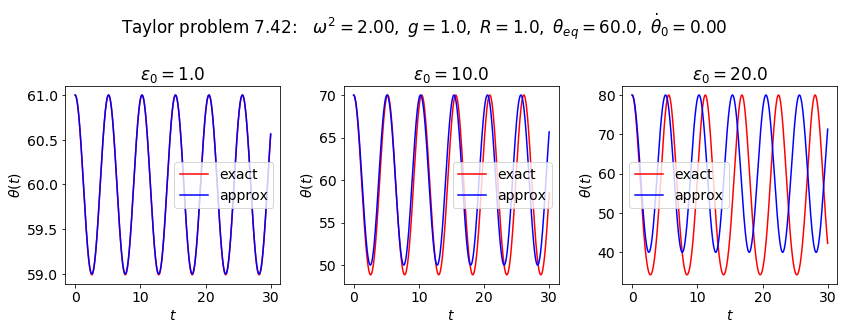
overall_title = 'Taylor problem 7.42: ' + \
rf' $\omega^2 = {omega**2:.2f},$' + \
rf' $g = {g:.1f},$' + \
rf' $R = {R:.1f},$' + \
rf' $\theta_{{eq}} = {o1.theta_equil * rad_to_deg:.1f},$' + \
rf' $\dot\theta_0 = {theta_dot_0:.2f}$' + \
'\n' # \n means a new line (adds some space here)
fig.suptitle(overall_title, va='baseline')
# plot 1
epsilon_0 = 1. * deg_to_rad
theta_0 = o1.theta_equil + epsilon_0
theta_dot_0 = 0.0
theta, theta_dot = o1.solve_ode(t_pts, theta_0, theta_dot_0)
theta_approx = o1.small_angle(t_pts, epsilon_0)
ax_a = fig.add_subplot(1,3,1)
start, stop = start_stop_indices(t_pts, 0., 30.)
plot_y_vs_x(t_pts[start : stop], theta[start : stop] * rad_to_deg,
axis_labels=theta_vs_time_labels,
color='red',
label='exact',
ax=ax_a)
plot_y_vs_x(t_pts[start : stop], theta_approx[start : stop] * rad_to_deg,
axis_labels=theta_vs_time_labels,
color='blue',
label='approx',
title=rf'$\epsilon_0={epsilon_0*rad_to_deg:.1f}$',
ax=ax_a)
# plot 2
epsilon_0 = 10. * deg_to_rad
theta_0 = o1.theta_equil + epsilon_0
theta_dot_0 = 0.0
theta, theta_dot = o1.solve_ode(t_pts, theta_0, theta_dot_0)
theta_approx = o1.small_angle(t_pts, epsilon_0)
ax_b = fig.add_subplot(1,3,2)
start, stop = start_stop_indices(t_pts, 0., 30.)
plot_y_vs_x(t_pts[start : stop], theta[start : stop] * rad_to_deg,
axis_labels=theta_vs_time_labels,
color='red',
label='exact',
ax=ax_b)
plot_y_vs_x(t_pts[start : stop], theta_approx[start : stop] * rad_to_deg,
axis_labels=theta_vs_time_labels,
color='blue',
label='approx',
title=rf'$\epsilon_0={epsilon_0*rad_to_deg:.1f}$',
ax=ax_b)
# plot 3
epsilon_0 = 20. * deg_to_rad
theta_0 = o1.theta_equil + epsilon_0
theta_dot_0 = 0.0
theta, theta_dot = o1.solve_ode(t_pts, theta_0, theta_dot_0)
theta_approx = o1.small_angle(t_pts, epsilon_0)
ax_b = fig.add_subplot(1,3,3)
start, stop = start_stop_indices(t_pts, 0., 30.)
plot_y_vs_x(t_pts[start : stop], theta[start : stop] * rad_to_deg,
axis_labels=theta_vs_time_labels,
color='red',
label='exact',
ax=ax_b)
plot_y_vs_x(t_pts[start : stop], theta_approx[start : stop] * rad_to_deg,
axis_labels=theta_vs_time_labels,
color='blue',
label='approx',
title=rf'$\epsilon_0={epsilon_0*rad_to_deg:.1f}$',
ax=ax_b)
fig.tight_layout()
fig.savefig('Taylor_problem_7.42.png', bbox_inches='tight')