Sine map explorations (Taylor and beyond)
Contents
Sine map explorations (Taylor and beyond)#
Modified version of Logistic_map_explorations.ipynb, which in turn was adapted by Dick Furnstahl from the Ipython Cookbook by Cyrille Rossant.
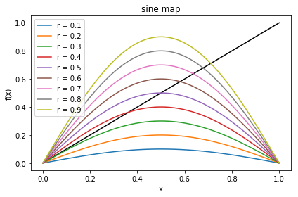
Here we consider the sine map. The defining function for the sine map is
\( f_r(x) = r \sin(\pi x) \;, \)
where \(r\) is the control parameter analogous to \(\gamma\) for the damped, driven pendulum. To study the pendulum, we looked at \(\phi(t)\) at \(t_0\), \(t_0 + \tau\), \(t_0 + 2\tau\), and so on, where \(\tau\) is the driving frequency and we found \(\phi(t_0 + \tau)\) from \(\phi(t_0)\) by solving the differential equation for the pendulum. After transients had died off, we characterized the value of \(\gamma\) being considered by the periodicity of the \(\phi(t_n)\) values: period one (all the same), period two (alternating), chaotic (no repeats) and so on.
Here instead of a differential equation telling us how to generate a trajectory, we use \(f_r(x)\):
\(\begin{align} x_1 = f_r(x_0) \ \rightarrow\ x_2 = f_r(x_1) \ \rightarrow\ x_3 = f_r(x_2) \ \rightarrow\ \ldots \end{align}\)
There will be transients at the beginning, but this sequence of \(x_i\) values may reach a point \(x = x^*\) such that \(f(x^*) = x^*\). We call this a fixed point. If instead it ends up bouncing between two values of \(x\), it is period two and we call it a two-cycle. We can have a cascade of period doubling, as found for the damped, driven pendulum, leading to chaos, which is characterized by the mapping never repeating. We can make a corresponding bifurcation diagram and identify Lyapunov exponents for each initial condition and \(r\).
%matplotlib inline

# standard numpy and matplotlib imports
import numpy as np
import matplotlib.pyplot as plt
def sine_map(r, x):
    """Sine map function: f_r(x) = r sin(pi x)
    """
    return r * np.sin(np.pi * x)

def sine_map_deriv(r, x):
    """Sine map derivative: f'(x) = r(1-2x)
    """
    return r * np.pi * np.cos(np.pi * x)
Explore the sine map and its fixed points#
Start with a simple plot of the sine function for \(0.1 \leq r \leq 0.9\).
x_pts, step = np.linspace(0,1, num=101, endpoint=True, retstep=True)
fig = plt.figure()
ax = fig.add_subplot(1,1,1)

ax.plot(x_pts, x_pts, color='black')

r_pts = np.arange(.1, 1., .1)
for r in r_pts:
    ax.plot(x_pts, sine_map(r, x_pts), label=rf'r = {r:.1f}')
ax.legend()

ax.set_xlabel('x')
ax.set_ylabel('f(x)')
ax.set_title('sine map')

fig.tight_layout()
fig.savefig('problem_12.23a.png', bbox_inches='tight')
Make plots showing the approach to fixed points.
Play with the number of steps taken and the values of \(r\).
Increase the number of steps in the plots to more cleanly identify the long-time trend for that value of \(r\).
Try smaller values of \(r\). Are there always non-zero fixed points for small \(r\)?
def plot_system(r, x0, n, ax=None):
    """Plot the function and the y=x diagonal line."""
    t = np.linspace(0,1, num=101)
    ax.plot(t, sine_map(r,t), 'k', lw=2)  # black, linewidth 2
    ax.plot([0,1], [0,1], 'k', lw=2)  # x is an array of 0 and 1,
                                      # y is the same array, so this plots
                                      #  a straight line from (0,0) to (1,1).

    # Recursively apply y=f(x) and plot two additional straight lines:
    #   line from (x, x) to (x, y)
    #   line from (x, y) to (y, y)
    x = x0
    for i in range(n):   # do n iterations, i = 0, 1, ..., n-1
        y = sine_map(r, x)
        # Plot the two lines
        ax.plot([x,x], [x,y], color='blue', lw=1)
        ax.plot([x,y], [y,y], color='blue', lw=1)
        # Plot the positions with increasing opacity of the circles
        ax.plot([x], [y], 'or', ms=10, alpha=(i+1)/n)
        x = y  # recursive: reset x to y for the next iteration
    ax.set_xlim(0,1)
    ax.set_ylim(0,1)
    ax.set_title(f'$r={r:.2f}$, $x_0={x0:.1f}$')
    ax.set_xlabel('x')

fig = plt.figure(figsize=(12,12))

ax1 = fig.add_subplot(2,2,1)
# start at 0.1, take n steps
plot_system(r=0.6, x0=0.1, n=10, ax=ax1)

ax2 = fig.add_subplot(2,2,2)
# start at 0.1, take n steps
plot_system(r=0.8, x0=0.1, n=20, ax=ax2)

ax3 = fig.add_subplot(2,2,3)
# start at 0.1, take n steps
plot_system(r=0.85, x0=0.1, n=40, ax=ax3)

ax4 = fig.add_subplot(2,2,4)
# start at 0.1, take n steps
plot_system(r=0.9, x0=0.1, n=40, ax=ax4)

fig.savefig('problem_12.23b.png', bbox_inches='tight')
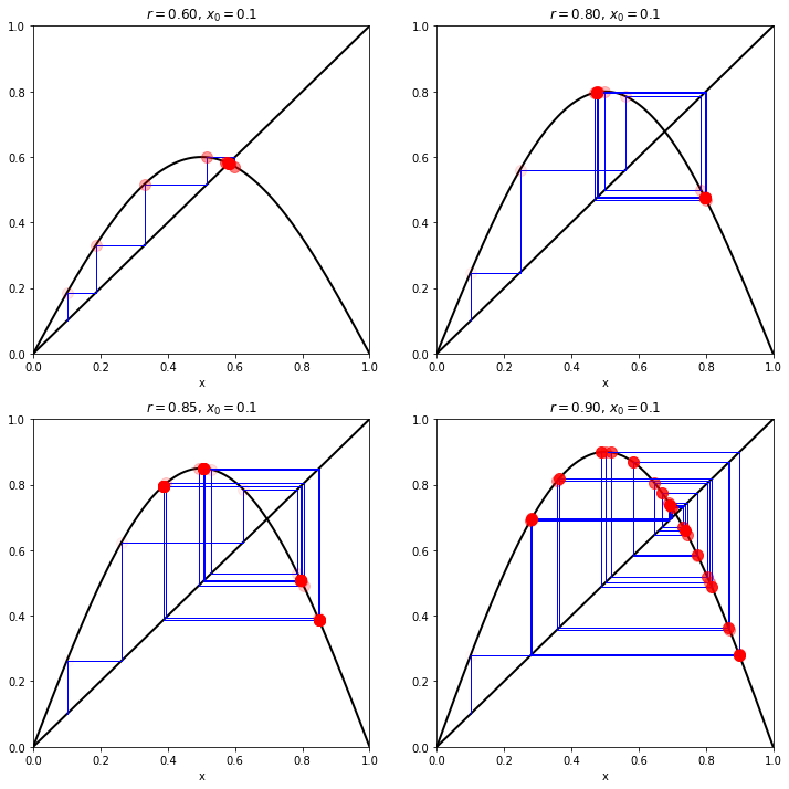
What periods do these exhibit? Are any chaotic?
\(r=0.6\) is period one, \(r=0.8\) is period 2, \(r=0.85\) is period 4, \(r=0.9\) is apparently chaotic.
Find the unstable point numerically#
To find the value of \(r\) at which the second fixed point becomes unstable, we must solve simultaneously the equations (see Taylor 12.9 in the “A Test for Stability” subsection):
\(\begin{align} &f_r(x^*) = x^* \\ &f_r'(x^*) = -1 \end{align}\)
where \(f'\) means the derivative with respect to \(x\), or
\(\begin{align} &f_r(x^*) - x^* = 0 \\ &f_r'(x^*) + 1 = 0 \end{align}\)
It is the latter form of the equations that we will pass to the
scipy function fsolve to find the values of \(r\) and \(x*\).
from scipy.optimize import fsolve  # Google this to learn more!

def equations(passed_args):
    """Return the two expressions that must equal to zero."""
    r, x = passed_args
    return (sine_map(r, x) - x, sine_map_deriv(r, x) + 1)

# Call fsolve with initial values for r and x
r, x = fsolve(equations, (0.5, 0.5))

print_string = f'x* = {x:.10f},  r = {r:.10f}'
print(print_string)
x* = 0.6457736765, r = 0.7199616829
Verify analytically that these are the correct values for the logistic map. We use this same procedure for other maps where only numerical solutions are known.
Now make the bifurcation diagram and calculate Lyapunov exponents#
To make a bifurcation diagram, we:
define an array of closely spaced \(r\) values;
for each \(r\), iterate the map \(x_{i+1} = f_r(x_i)\) a large number of times (e.g., 1000) to ensure convergence;
plot the last 100 or so iterations as points at each \(r\).
To think about how to calculate a Lyapunov exponent, consider two iterations of the map starting from two values of \(x\) that are close together. Call these initial values \(x_0\) and \(x_0 + \delta x_0\). These are mapped by \(f_r\) to \(x_1\) and \(x_1 + \delta x_1\), then \(x_2\) and \(x_2 + \delta x_2\), up to \(x_n + \delta x_n\).
How are the \(\delta x_i\) related? Each \(\delta x_i\) is small, so use a Taylor expansion! Expanding \(f(x)\) about \(x_n\):
\(\begin{align} f(x_i &+ \delta x_i) = &f(x_i) + \delta x_i f'(x_i) + \frac{1}{2}(\delta x_i)^2 f''(x_i) + \cdots \\ \end{align}\)
so, neglecting terms of order \((\delta x_i)^2\) and higher,
\(\begin{align} x_{i+1} + \delta x_{i+1} \approx x_{i+1} + \delta x_i f'(x_i) \quad\mbox{or}\quad \delta x_{i+1} \approx f'(x_i)\, \delta x_i \;. \end{align}\)
Iterating this result we get
\(\begin{align} \delta x_1 &= f'(x_0)\, \delta x_0 \\ \delta x_2 &= f'(x_1)\, \delta x_1 = f'(x_1)\times f'(x_0)\, \delta x_0 \\ & \qquad\vdots \\ |\delta x_n| &= \left(\prod_{i=0}^{n-1} |f'(x_i)|\right) |\delta x_0| \;, \end{align}\)
where the last equation gives us the separation of two trajectories after \(n\) steps \(\delta x_n\) in terms of their initial separation, \(\delta x_0\). (Why can we just take the absolute value of all the terms?)
We expect that this will vary exponentially at large \(n\) like
\(\begin{align} \left| \frac{\delta x_n}{\delta x_0} \right| = e^{\lambda n} \end{align}\)
and so we define the Lypunov exponent \(\lambda\) by
\(\begin{align} \lambda = \lim_{n\rightarrow\infty} \frac{1}{n} \sum_{i=1}^{n} \ln |f'(x_i)| \;, \end{align}\)
which in practice is well approximated by the sum for large \(n\).
If \(\lambda > 0\), then nearby trajectories diverge from each other exponentially at large \(n\), which corresponds to chaos. However, if the trajectories converge to a fixed point or a limit cycle, they will get closer together with increasing \(n\), which corresponds to \(\lambda<0\).
Ok, let’s do it!
n = 10000
# Here we'll use n values of r linearly spaced between 2.8 and 4.0
###  You may want to change the range of r for other maps
r = np.linspace(0.6, 1.0, n)

iterations = 1000   # iterations of logistic map; keep last iterations
last = 100          #  where results should have stabilized

x = 0.1 * np.ones(n)  # x_0 initial condition
                      ### (you may want to change for other maps)

lyapunov = np.zeros(n) # initialize vector used for the Lyapunov sums
fig = plt.figure(figsize=(8,9))
ax1 = fig.add_subplot(2,1,1)   # bifurcation diagram
ax2 = fig.add_subplot(2,1,2)   # Lyapunov exponent

# Display the bifurcation diagram with one pixel per point x_n^(r) for last iterations
for i in range(iterations):
    x = sine_map(r,x)  # just iterate: x_{i+1} = f_r(x_i)

    # Compute the partial sum of the Lyapunov exponent, which is the sum
    #  of derivatives of the logistic function (absolute value)
    lyapunov += np.log(abs(sine_map_deriv(r,x)))
    # Display the bifurcation diagram.
    if i >= (iterations-last):  # only plot the last iterations
        ax1.plot(r, x, ',k', alpha=0.25)
ax1.set_xlim(0.6, 1.)
ax1.set_xlabel(r'$r$')
ax1.set_title("Bifurcation")

# Display the Lyapunov exponent

# Negative Lyapunov exponent
ax2.plot(r[lyapunov < 0],
         lyapunov[lyapunov < 0] / iterations, 'o',
         color='black', alpha=0.5, ms=0.5)
# Positive Lyapunov exponent
ax2.plot(r[lyapunov >= 0],
         lyapunov[lyapunov >= 0] / iterations, 'o',
         color='red', alpha=0.5, ms=0.5)

# Add a zero line (lightened with alpha=0.5)
ax2.axhline(0, color='k', lw=0.5, alpha=0.5)

ax2.set_xlim(0.6, 1.)
ax2.set_ylim(-2, 1.5)
ax2.set_xlabel(r'$r$')
ax2.set_title("Lyapunov exponent")

fig.tight_layout()
fig.savefig('problem_12.34.png', bbox_inches='tight')
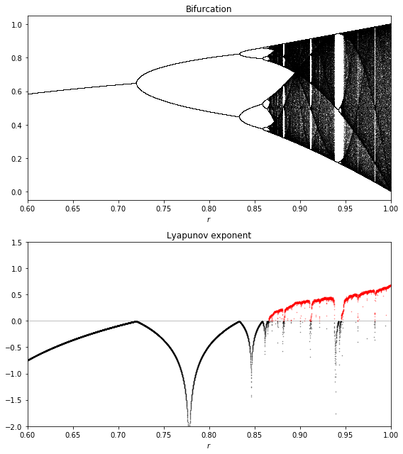
We see there is a fixed point for \(r < 3\), then two and four periods and a chaotic behavior when \(r\) belongs to certain areas of the parameter space. Do the values of \(r\) where these behaviors occur agree with what you found in the plots with particular \(r\) values?
As for the pendulum, the Lyapunov exponent is positive when the system is chaotic (in red). Do these regions look consistent with the characteristics of chaos?