Animating a simple wave

We’ll plot at various times a wave \(u(x,t)\) that starts as a triangular shape as in Taylor Example 16.1, and then animate it. We can imagine this as simulating a wave on a taut string. Here \(u\) is the transverse displacement (i.e., \(y\) in our two-dimensional plots). We are not solving the wave equation as a differential equation here, but starting with \(u(x,0) \equiv u_0(x)\) and plotting the solution at time \(t\):

\(\begin{align} u(x,t) = \frac12 u_0(x - ct) + \frac12 u_0(x + ct) \;, \end{align}\)

which is the solution to the wave equation starting with \(u_0(x)\) at time \(t=0\).

We have various choices for animation in a Jupyter notebook. We will consider two possibilities, which both use FuncAnimation from matplotlib.animation.

1. Make a javascript movie that is then displayed inline with a movie-playing widget using HTML. We use %matplotlib inline for this option and use %%capture to prevent the figure from displaying prematurely.

2. Update the figure in real time (so to speak) by using %matplotlib notebook, which creates active figures that we can modify after they are displayed.

We’ll do the first option here. We should define at least one class for the animation.

v1: Created 25-Mar-2019. Last revised 27-Mar-2019 by Dick Furnstahl (furnstahl.1@osu.edu).

%matplotlib inline

To use option 2: uncomment %matplotlib notebook here and fig.show() just after we define anim. Comment out %%capture and HTML(anim.to_jshtml()) below.

#%matplotlib notebook

import numpy as np
import matplotlib.pyplot as plt

from matplotlib import animation, rc
from IPython.display import HTML

First define functions for the \(t=0\) wave function form (here a triangle) and for the subsequent shape at any time \(t\) based on the wave speed c_wave.

def u_0_triangle(x_pts, height=1., width=1.):
    """Returns a triangular wave of amplitude height and width 2*width.  
    """
    y_pts = np.zeros(len(x_pts))  # set the y array to all zeros
    for i, x in enumerate(x_pts):
        if x < width and x >= 0.:
            y_pts[i] = -(height/width) * x + height
        elif x < 0 and x >= -width:
            y_pts[i] = (height/width) * x + height
        else:
            pass   # do nothing (everything else is zero already)
    return y_pts

def u_triangle(x_pts, t, c_wave = 1., height=1., width=1.):
    """Returns the wave at time t resulting from a triangular wave of 
       amplitude height and width 2*width at time t=0.  It is the
       superposition of two traveling waves moving to the left and the right.
    """
    y_pts = u_0_triangle(x_pts - c_wave * t) / 2. + \
            u_0_triangle(x_pts + c_wave * t) / 2.
    return y_pts

# Set up the array of x points (whatever looks good)
x_min = -5.
x_max = +5.
delta_x = 0.01
x_pts = np.arange(x_min, x_max, delta_x)

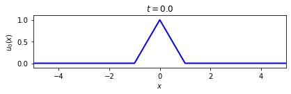
First look at the initial (\(t=0\)) wave form.

# Define the initial (t=0) wave form and the wave speed.
height = 1.
width = 1.
c_wave = 1.

# Make a figure showing the initial wave.
t_now = 0.

fig = plt.figure(figsize=(6,2), num='Triangular wave')
ax = fig.add_subplot(1,1,1)
ax.set_xlim(x_min, x_max)
gap = 0.1
ax.set_ylim(-gap, height + gap)
ax.set_xlabel(r'$x$')
ax.set_ylabel(r'$u_0(x)$')
ax.set_title(rf'$t = {t_now:.1f}$')

line, = ax.plot(x_pts, 
                u_triangle(x_pts, t_now, c_wave, height, width), 
                color='blue', lw=2)

fig.tight_layout()

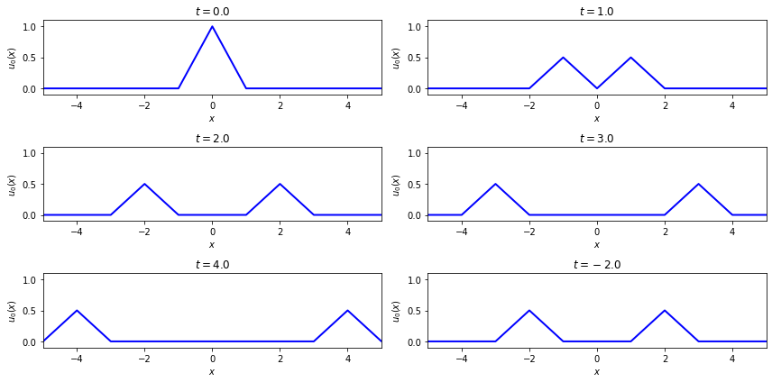
Next make some plots at an array of time points.

t_array = np.array([0., 1,  2.,  3,  4.,  -2.])

fig_array = plt.figure(figsize=(12,6), num='Triangular wave')

for i, t_now in enumerate(t_array): 
    ax_array = fig_array.add_subplot(3, 2, i+1)
    ax_array.set_xlim(x_min, x_max)
    gap = 0.1
    ax_array.set_ylim(-gap, height + gap)
    ax_array.set_xlabel(r'$x$')
    ax_array.set_ylabel(r'$u_0(x)$')
    ax_array.set_title(rf'$t = {t_now:.1f}$')

    ax_array.plot(x_pts, 
                  u_triangle(x_pts, t_now, c_wave, height, width), 
                  color='blue', lw=2)

fig_array.tight_layout()
fig_array.savefig('Taylor_Example_16p1_triangle_waves.png', 
                   bbox_inches='tight')  

Now it is time to animate!

# Set up the t mesh for the animation.  The maximum value of t shown in
#  the movie will be t_min + delta_t * frame_number
t_min = 0.   # You can make this negative to see what happens before t=0!
t_max = 15.
delta_t = 0.1
t_pts = np.arange(t_min, t_max, delta_t)

We use the cell “magic” %%capture to keep the figure from being shown here. If we didn’t the animated version below would be blank.

%%capture

fig_anim = plt.figure(figsize=(6,2), num='Triangular wave')
ax_anim = fig_anim.add_subplot(1,1,1)
ax_anim.set_xlim(x_min, x_max)
gap = 0.1
ax_anim.set_ylim(-gap, height + gap)

# By assigning the first return from plot to line_anim, we can later change
#  the values in the line.
line_anim, = ax_anim.plot(x_pts, 
                          u_triangle(x_pts, t_min, c_wave, height, width), 
                          color='blue', lw=2)

fig_anim.tight_layout()

def animate_wave(i):
    """This is the function called by FuncAnimation to create each frame,
        numbered by i.  So each i corresponds to a point in the t_pts
        array, with index i.
    """
    t = t_pts[i]
    y_pts = u_triangle(x_pts, t, c_wave, height, width) 

    line_anim.set_data(x_pts, y_pts)  # overwrite line_anim with new points
    return (line_anim,)   # this is needed for blit=True to work

frame_interval = 40.  # time between frames
frame_number = 100    # number of frames to include (index of t_pts)
anim = animation.FuncAnimation(fig_anim, 
                               animate_wave, 
                               init_func=None,
                               frames=frame_number, 
                               interval=frame_interval, 
                               blit=True,
                               repeat=False)

#fig.show()

HTML(anim.to_jshtml())

Once Loop Reflect