Multiple pendulum plots: Section 12.3
Contents
Multiple pendulum plots: Section 12.3#
Use Pendulum class to generate basic pendulum plots. Applied here to examples from Taylor Section 12.3.
Last revised 21-Jan-2019 by Dick Furnstahl (furnstahl.1@osu.edu).
%matplotlib inline
import numpy as np
from scipy.integrate import odeint

import matplotlib.pyplot as plt
Pendulum class and utility functions#
class Pendulum():
    """
    Pendulum class implements the parameters and differential equation for
     a pendulum using the notation from Taylor.

    Parameters
    ----------
    omega_0 : float
        natural frequency of the pendulum (\sqrt{g/l} where l is the
        pendulum length)
    beta : float
        coefficient of friction
    gamma_ext : float
        amplitude of external force is gamma * omega_0**2
    omega_ext : float
        frequency of external force
    phi_ext : float
        phase angle for external force

    Methods
    -------
    dy_dt(y, t)
        Returns the right side of the differential equation in vector y,
        given time t and the corresponding value of y.
    driving_force(t)
        Returns the value of the external driving force at time t.
    """
    def __init__(self, omega_0=1., beta=0.2,
                 gamma_ext=0.2, omega_ext=0.689, phi_ext=0.
                ):
        self.omega_0 = omega_0
        self.beta = beta
        self.gamma_ext = gamma_ext
        self.omega_ext = omega_ext
        self.phi_ext = phi_ext

    def dy_dt(self, y, t):
        """
        This function returns the right-hand side of the diffeq:
        [dphi/dt d^2phi/dt^2]

        Parameters
        ----------
        y : float
            A 2-component vector with y[0] = phi(t) and y[1] = dphi/dt
        t : float
            time

        Returns
        -------

        """
        F_ext = self.driving_force(t)
        return [y[1], -self.omega_0**2 * np.sin(y[0]) - 2.*self.beta * y[1] \
                       + F_ext]

    def driving_force(self, t):
        """
        This function returns the value of the driving force at time t.
        """
        return self.gamma_ext * self.omega_0**2 \
                              * np.cos(self.omega_ext*t + self.phi_ext)

    def solve_ode(self, phi_0, phi_dot_0, abserr=1.0e-8, relerr=1.0e-6):
        """
        Solve the ODE given initial conditions.
        For now use odeint, but we have the option to switch.
        Specify smaller abserr and relerr to get more precision.
        """
        y = [phi_0, phi_dot_0]
        phi, phi_dot = odeint(self.dy_dt, y, t_pts,
                              atol=abserr, rtol=relerr).T
        return phi, phi_dot
def plot_y_vs_x(x, y, axis_labels=None, label=None, title=None,
                color=None, linestyle=None, semilogy=False, loglog=False,
                ax=None):
    """
    Generic plotting function: return a figure axis with a plot of y vs. x,
    with line color and style, title, axis labels, and line label
    """
    if ax is None:        # if the axis object doesn't exist, make one
        ax = plt.gca()

    if (semilogy):
        line, = ax.semilogy(x, y, label=label,
                            color=color, linestyle=linestyle)
    elif (loglog):
        line, = ax.loglog(x, y, label=label,
                          color=color, linestyle=linestyle)
    else:
        line, = ax.plot(x, y, label=label,
                    color=color, linestyle=linestyle)

    if label is not None:    # if a label if passed, show the legend
        ax.legend()
    if title is not None:    # set a title if one if passed
        ax.set_title(title)
    if axis_labels is not None:  # set x-axis and y-axis labels if passed
        ax.set_xlabel(axis_labels[0])
        ax.set_ylabel(axis_labels[1])

    return ax, line
def start_stop_indices(t_pts, plot_start, plot_stop):
    start_index = (np.fabs(t_pts-plot_start)).argmin()  # index in t_pts array
    stop_index = (np.fabs(t_pts-plot_stop)).argmin()  # index in t_pts array
    return start_index, stop_index
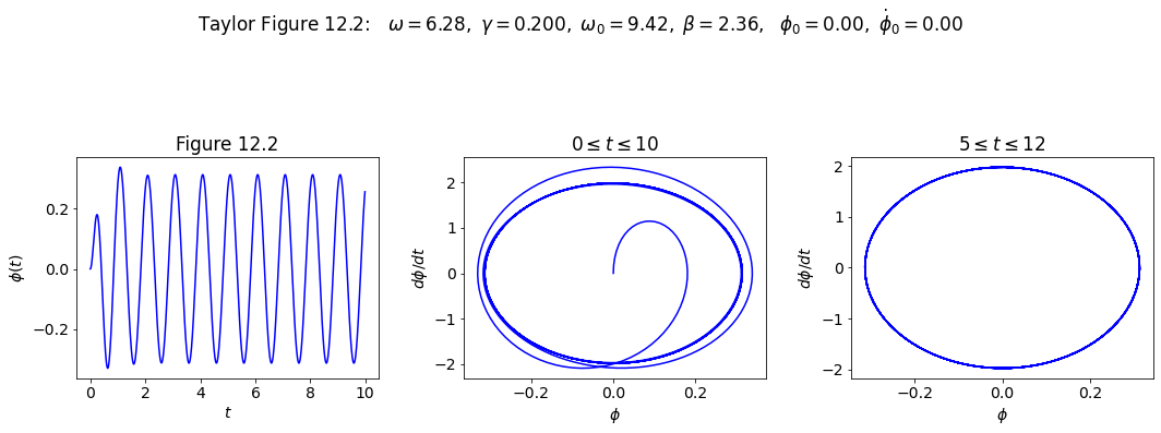
Make plots for Taylor Figure 12.2#
We’ll set it up with the specified parameters.
# Labels for individual plot axes
phi_vs_time_labels = (r'$t$', r'$\phi(t)$')
phi_dot_vs_time_labels = (r'$t$', r'$d\phi/dt(t)$')
state_space_labels = (r'$\phi$', r'$d\phi/dt$')

# Common plotting time (generate the full time then use slices)
t_start = 0.
t_end = 100.
delta_t = 0.01

t_pts = np.arange(t_start, t_end+delta_t, delta_t)

# Common pendulum parameters
gamma_ext = 0.2
omega_ext = 2.*np.pi
phi_ext = 0.

omega_0 = 1.5*omega_ext
beta = omega_0/4.

# Instantiate a pendulum
p1 = Pendulum(omega_0=omega_0, beta=beta,
              gamma_ext=gamma_ext, omega_ext=omega_ext, phi_ext=phi_ext)

# calculate the driving force for t_pts
driving = p1.driving_force(t_pts)
# initial conditions specified
phi_0 = 0.
phi_dot_0 = 0.0
phi, phi_dot = p1.solve_ode(phi_0, phi_dot_0)

# Change the common font size
font_size = 14
plt.rcParams.update({'font.size': font_size})

# start the plot!
fig = plt.figure(figsize=(15,5))
overall_title = 'Taylor Figure 12.2:  ' + \
                rf' $\omega = {omega_ext:.2f},$' + \
                rf' $\gamma = {gamma_ext:.3f},$' + \
                rf' $\omega_0 = {omega_0:.2f},$' + \
                rf' $\beta = {beta:.2f},$' + \
                rf'  $\phi_0 = {phi_0:.2f},$' + \
                rf' $\dot\phi_0 = {phi_dot_0:.2f}$' + \
                '\n'     # \n means a new line (adds some space here)
fig.suptitle(overall_title, va='baseline')

# first plot: plot from t=0 to t=10
ax_a = fig.add_subplot(1,3,1)

start, stop = start_stop_indices(t_pts, 0., 10.)
plot_y_vs_x(t_pts[start : stop], phi[start : stop],
            axis_labels=phi_vs_time_labels,
            color='blue',
            label=None,
            title='Figure 12.2',
            ax=ax_a)

# second plot: state space plot from t=0 to t=10
ax_b = fig.add_subplot(1,3,2)

start, stop = start_stop_indices(t_pts, 0., 10.)
plot_y_vs_x(phi[start : stop], phi_dot[start : stop],
            axis_labels=state_space_labels,
            color='blue',
            label=None,
            title=rf'$0 \leq t \leq 10$',
            ax=ax_b)

# third plot: state space plot from t=5 to t=12
ax_c = fig.add_subplot(1,3,3)

start, stop = start_stop_indices(t_pts, 5., 12.)
plot_y_vs_x(phi[start : stop], phi_dot[start : stop],
            axis_labels=state_space_labels,
            color='blue',
            label=None,
            title=rf'$5 \leq t \leq 12$',
            ax=ax_c)

fig.tight_layout()
fig.savefig('Figure_12.2.png', bbox_inches='tight')  # always bbox_inches='tight'
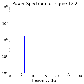
Now trying the power spectrum in steady state, plotting only positive frequencies and cutting off any lower peaks from noise. We multiply the frequencies by \(2\pi\) to get the angular frequency. What do you observe?
start, stop = start_stop_indices(t_pts, 20., t_end)
signal = phi[start:stop]
power_spectrum = np.abs(np.fft.fft(signal))**2
freqs = 2.*np.pi * np.fft.fftfreq(signal.size, delta_t)
idx = np.argsort(freqs)

fig_ps = plt.figure(figsize=(5,5))
ax_ps = fig_ps.add_subplot(1,1,1)
ax_ps.semilogy(freqs[idx], power_spectrum[idx], color='blue')
ax_ps.set_xlim(0, 30.)
ax_ps.set_ylim(1.e4, 1.e8)
ax_ps.set_xlabel('frequency (Hz)')
ax_ps.set_title('Power Spectrum for Figure 12.2')

fig_ps.tight_layout()
Sections 12.1 \(--\) 12.3 Q1: Pick conditions and then analyze#
# Labels for individual plot axes
phi_vs_time_labels = (r'$t$', r'$\phi(t)$')
phi_dot_vs_time_labels = (r'$t$', r'$d\phi/dt(t)$')
state_space_labels = (r'$\phi$', r'$d\phi/dt$')

# Common plotting time (generate the full time then use slices)
t_start = 0.
t_end = 100.
delta_t = 0.01

t_pts = np.arange(t_start, t_end+delta_t, delta_t)

# Common pendulum parameters
gamma_ext = 0.01   # weak driving
omega_ext = 2.*np.pi
phi_ext = np.pi/2.  # come back to this later!

omega_0 = 1.5*omega_ext
beta = omega_0/10.  # weak damping

# Instantiate a pendulum
p1 = Pendulum(omega_0=omega_0, beta=beta,
              gamma_ext=gamma_ext, omega_ext=omega_ext, phi_ext=phi_ext)

# calculate the driving force for t_pts
driving = p1.driving_force(t_pts)
# initial conditions specified
phi_0 = np.pi    # at the top
phi_dot_0 = 0.0  # motionless
phi, phi_dot = p1.solve_ode(phi_0, phi_dot_0)

# Change the common font size
font_size = 14
plt.rcParams.update({'font.size': font_size})

# start the plot!
fig = plt.figure(figsize=(15,5))
overall_title = 'Taylor Figure 12.2:  ' + \
                rf' $\omega = {omega_ext:.2f},$' + \
                rf' $\gamma = {gamma_ext:.3f},$' + \
                rf' $\omega_0 = {omega_0:.2f},$' + \
                rf' $\beta = {beta:.2f},$' + \
                rf'  $\phi_0 = {phi_0:.2f},$' + \
                rf' $\dot\phi_0 = {phi_dot_0:.2f}$' + \
                '\n'     # \n means a new line (adds some space here)
fig.suptitle(overall_title, va='baseline')

# first plot: plot from t=0 to t=20
ax_a = fig.add_subplot(1,3,1)

start, stop = start_stop_indices(t_pts, 0., 20.)
plot_y_vs_x(t_pts[start : stop], phi[start : stop],
            axis_labels=phi_vs_time_labels,
            color='blue',
            label=None,
            title='Q1',
            ax=ax_a)

# second plot: same as first but scaled up
ax_b = fig.add_subplot(1,3,2)

start, stop = start_stop_indices(t_pts, 0., 20.)
plot_y_vs_x(t_pts[start : stop], phi[start : stop],
            axis_labels=phi_vs_time_labels,
            color='blue',
            label=None,
            title='Q1',
            ax=ax_b)
ax_b.set_ylim(-0.07, 0.07)

# third plot: state space plot from t=0 to t=7
ax_c = fig.add_subplot(1,3,3)

start, stop = start_stop_indices(t_pts, 0., 7.)
plot_y_vs_x(phi[start : stop], phi_dot[start : stop],
            axis_labels=state_space_labels,
            color='blue',
            label=None,
            title=rf'$0 \leq t \leq 7$',
            ax=ax_c)

fig.tight_layout()
fig.savefig('Section_12.3_Q1.png', bbox_inches='tight')  # always bbox_inches='tight'
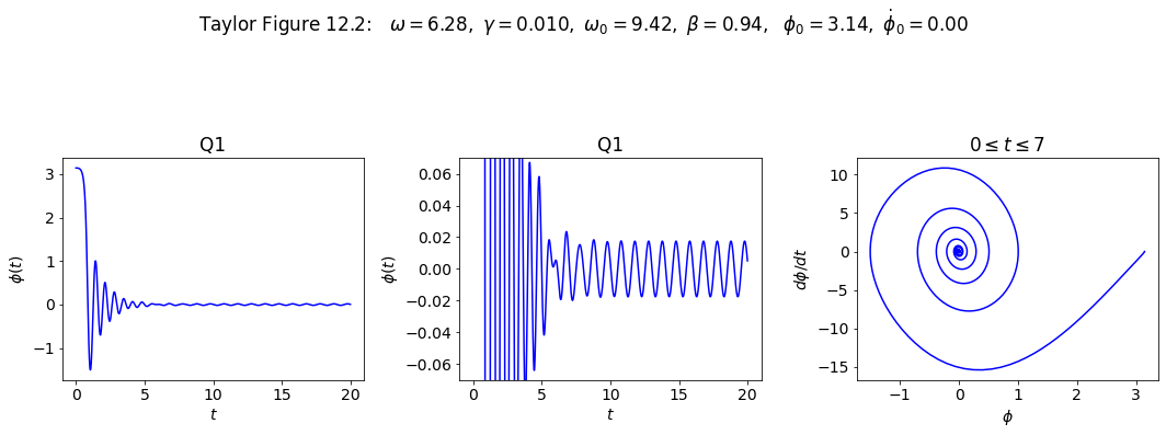
Now go back and predict what the state space plot will look like if we skip the transient region.
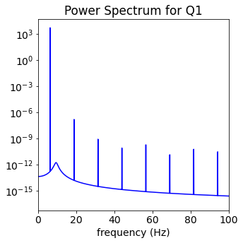
Now trying the power spectrum in steady state, plotting only positive frequencies and cutting off any lower peaks from noise. We multiply the frequencies by \(2\pi\) to get the angular frequency. What do you observe?
start, stop = start_stop_indices(t_pts, 20., t_end)
signal = phi[start:stop]
power_spectrum = np.abs(np.fft.fft(signal))**2
freqs = 2.*np.pi * np.fft.fftfreq(signal.size, delta_t)
idx = np.argsort(freqs)

fig_ps = plt.figure(figsize=(5,5))
ax_ps = fig_ps.add_subplot(1,1,1)
ax_ps.semilogy(freqs[idx], power_spectrum[idx], color='blue')
ax_ps.set_xlim(0, 100.)
#ax_ps.set_ylim(1.e4, 1.e8)
ax_ps.set_xlabel('frequency (Hz)')
ax_ps.set_title('Power Spectrum for Q1')

fig_ps.tight_layout()
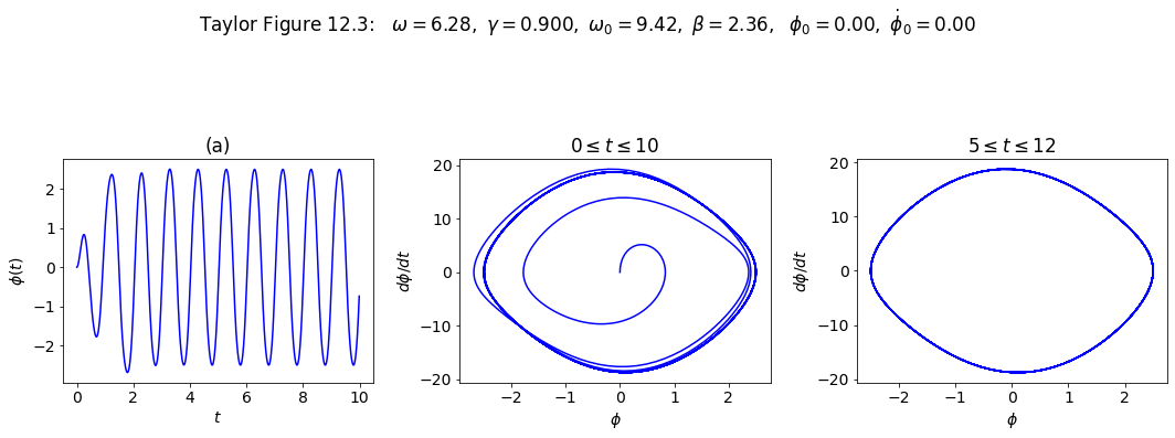
Make plots for Taylor Figure 12.3#
Just change \(\gamma\) from 0.2 to 0.9 compared to Figure 12.2.
# Labels for individual plot axes
phi_vs_time_labels = (r'$t$', r'$\phi(t)$')
phi_dot_vs_time_labels = (r'$t$', r'$d\phi/dt(t)$')
state_space_labels = (r'$\phi$', r'$d\phi/dt$')

# Common plotting time (generate the full time then use slices)
t_start = 0.
t_end = 100.
delta_t = 0.01

t_pts = np.arange(t_start, t_end+delta_t, delta_t)

# Common pendulum parameters
gamma_ext = 0.9
omega_ext = 2.*np.pi
phi_ext = 0.

omega_0 = 1.5*omega_ext
beta = omega_0/4.

# Instantiate a pendulum
p1 = Pendulum(omega_0=omega_0, beta=beta,
              gamma_ext=gamma_ext, omega_ext=omega_ext, phi_ext=phi_ext)

# calculate the driving force for t_pts
driving = p1.driving_force(t_pts)
# initial conditions specified
phi_0 = 0.
phi_dot_0 = 0.0
phi, phi_dot = p1.solve_ode(phi_0, phi_dot_0)

# Change the common font size
font_size = 14
plt.rcParams.update({'font.size': font_size})

# start the plot!
fig = plt.figure(figsize=(15,5))
overall_title = 'Taylor Figure 12.3:  ' + \
                rf' $\omega = {omega_ext:.2f},$' + \
                rf' $\gamma = {gamma_ext:.3f},$' + \
                rf' $\omega_0 = {omega_0:.2f},$' + \
                rf' $\beta = {beta:.2f},$' + \
                rf'  $\phi_0 = {phi_0:.2f},$' + \
                rf' $\dot\phi_0 = {phi_dot_0:.2f}$' + \
                '\n'     # \n means a new line (adds some space here)
fig.suptitle(overall_title, va='baseline')

# first plot: plot from t=0 to t=10
ax_a = fig.add_subplot(1,3,1)

start, stop = start_stop_indices(t_pts, 0., 10.)
plot_y_vs_x(t_pts[start : stop], phi[start : stop],
            axis_labels=phi_vs_time_labels,
            color='blue',
            label=None,
            title='(a)',
            ax=ax_a)

# second plot: state space plot from t=0 to t=10
ax_b = fig.add_subplot(1,3,2)

start, stop = start_stop_indices(t_pts, 0., 10.)
plot_y_vs_x(phi[start : stop], phi_dot[start : stop],
            axis_labels=state_space_labels,
            color='blue',
            label=None,
            title=rf'$0 \leq t \leq 10$',
            ax=ax_b)

# third plot: state space plot from t=5 to t=12
ax_c = fig.add_subplot(1,3,3)

start, stop = start_stop_indices(t_pts, 5., 12.)
plot_y_vs_x(phi[start : stop], phi_dot[start : stop],
            axis_labels=state_space_labels,
            color='blue',
            label=None,
            title=rf'$5 \leq t \leq 12$',
            ax=ax_c)

fig.tight_layout()
fig.savefig('Figure_12.3.png', bbox_inches='tight')  # always bbox_inches='tight'
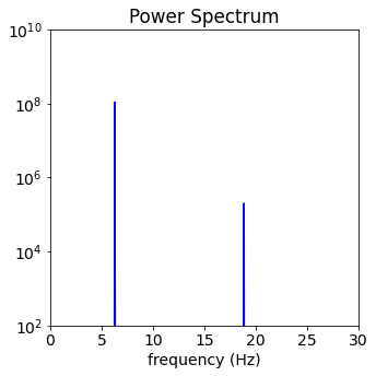
Now trying the power spectrum in steady state, plotting only positive frequencies and cutting off any lower peaks from noise. We multiply the frequencies by \(2\pi\) to get the angular frequency. What do you observe?
start, stop = start_stop_indices(t_pts, 20., t_end)
signal = phi[start:stop]
power_spectrum = np.abs(np.fft.fft(signal))**2
freqs = 2.*np.pi * np.fft.fftfreq(signal.size, delta_t)
idx = np.argsort(freqs)

fig_ps = plt.figure(figsize=(5,5))
ax_ps = fig_ps.add_subplot(1,1,1)
ax_ps.semilogy(freqs[idx], power_spectrum[idx], color='blue')
ax_ps.set_xlim(0, 30.)
ax_ps.set_ylim(1.e2, 1.e10)
ax_ps.set_xlabel('frequency (Hz)')
ax_ps.set_title('Power Spectrum')

fig_ps.tight_layout()