Multiple pendulum plots. Section 12.4: Approach to Chaos
Contents
Multiple pendulum plots. Section 12.4: Approach to Chaos#
Use Pendulum class to generate basic pendulum plots. Applied here to figures from Taylor Section 12.4.
Last revised 23-Jan-2019 by Dick Furnstahl (furnstahl.1@osu.edu).
%matplotlib inline
import numpy as np
from scipy.integrate import odeint

import matplotlib.pyplot as plt
Pendulum class and utility functions#
class Pendulum():
    """
    Pendulum class implements the parameters and differential equation for
     a pendulum using the notation from Taylor.

    Parameters
    ----------
    omega_0 : float
        natural frequency of the pendulum (\sqrt{g/l} where l is the
        pendulum length)
    beta : float
        coefficient of friction
    gamma_ext : float
        amplitude of external force is gamma * omega_0**2
    omega_ext : float
        frequency of external force
    phi_ext : float
        phase angle for external force

    Methods
    -------
    dy_dt(y, t)
        Returns the right side of the differential equation in vector y,
        given time t and the corresponding value of y.
    driving_force(t)
        Returns the value of the external driving force at time t.
    """
    def __init__(self, omega_0=1., beta=0.2,
                 gamma_ext=0.2, omega_ext=0.689, phi_ext=0.
                ):
        self.omega_0 = omega_0
        self.beta = beta
        self.gamma_ext = gamma_ext
        self.omega_ext = omega_ext
        self.phi_ext = phi_ext

    def dy_dt(self, y, t):
        """
        This function returns the right-hand side of the diffeq:
        [dphi/dt d^2phi/dt^2]

        Parameters
        ----------
        y : float
            A 2-component vector with y[0] = phi(t) and y[1] = dphi/dt
        t : float
            time

        Returns
        -------

        """
        F_ext = self.driving_force(t)
        return [y[1], -self.omega_0**2 * np.sin(y[0]) - 2.*self.beta * y[1] \
                       + F_ext]

    def driving_force(self, t):
        """
        This function returns the value of the driving force at time t.
        """
        return self.gamma_ext * self.omega_0**2 \
                              * np.cos(self.omega_ext*t + self.phi_ext)

    def solve_ode(self, phi_0, phi_dot_0, abserr=1.0e-8, relerr=1.0e-6):
        """
        Solve the ODE given initial conditions.
        For now use odeint, but we have the option to switch.
        Specify smaller abserr and relerr to get more precision.
        """
        y = [phi_0, phi_dot_0]
        phi, phi_dot = odeint(self.dy_dt, y, t_pts,
                              atol=abserr, rtol=relerr).T
        return phi, phi_dot
def plot_y_vs_x(x, y, axis_labels=None, label=None, title=None,
                color=None, linestyle=None, semilogy=False, loglog=False,
                ax=None):
    """
    Generic plotting function: return a figure axis with a plot of y vs. x,
    with line color and style, title, axis labels, and line label
    """
    if ax is None:        # if the axis object doesn't exist, make one
        ax = plt.gca()

    if (semilogy):
        line, = ax.semilogy(x, y, label=label,
                            color=color, linestyle=linestyle)
    elif (loglog):
        line, = ax.loglog(x, y, label=label,
                          color=color, linestyle=linestyle)
    else:
        line, = ax.plot(x, y, label=label,
                    color=color, linestyle=linestyle)

    if label is not None:    # if a label if passed, show the legend
        ax.legend()
    if title is not None:    # set a title if one if passed
        ax.set_title(title)
    if axis_labels is not None:  # set x-axis and y-axis labels if passed
        ax.set_xlabel(axis_labels[0])
        ax.set_ylabel(axis_labels[1])

    return ax, line
def start_stop_indices(t_pts, plot_start, plot_stop):
    """Given an array (e.g., of times) and desired starting and stop values,
        return the array indices that are closest to those values.
    """
    start_index = (np.fabs(t_pts-plot_start)).argmin()  # index in t_pts array
    stop_index = (np.fabs(t_pts-plot_stop)).argmin()  # index in t_pts array
    return start_index, stop_index
Make plots for Taylor Figure 12.4#
We’ll set it up with the specified parameters.
# Labels for individual plot axes
phi_vs_time_labels = (r'$t$', r'$\phi(t)$')
phi_dot_vs_time_labels = (r'$t$', r'$d\phi/dt(t)$')
state_space_labels = (r'$\phi$', r'$d\phi/dt$')

# Common plotting time (generate the full time then use slices)
t_start = 0.
t_end = 100.
delta_t = 0.01

t_pts = np.arange(t_start, t_end+delta_t, delta_t)

# Common pendulum parameters
gamma_ext = 1.06
omega_ext = 2.*np.pi
phi_ext = 0.

omega_0 = 1.5*omega_ext
beta = omega_0/4.

# Instantiate a pendulum
p1 = Pendulum(omega_0=omega_0, beta=beta,
              gamma_ext=gamma_ext, omega_ext=omega_ext, phi_ext=phi_ext)

# calculate the driving force for t_pts
driving = p1.driving_force(t_pts)
# initial conditions specified
phi_0 = 0.
phi_dot_0 = 0.0
phi, phi_dot = p1.solve_ode(phi_0, phi_dot_0)

# Change the common font size
font_size = 14
plt.rcParams.update({'font.size': font_size})

# start the plot!
fig = plt.figure(figsize=(15,5))
overall_title = 'Taylor Figure 12.4:  ' + \
                rf' $\omega = {omega_ext:.2f},$' + \
                rf' $\gamma = {gamma_ext:.3f},$' + \
                rf' $\omega_0 = {omega_0:.2f},$' + \
                rf' $\beta = {beta:.2f},$' + \
                rf'  $\phi_0 = {phi_0:.2f},$' + \
                rf' $\dot\phi_0 = {phi_dot_0:.2f}$' + \
                '\n'     # \n means a new line (adds some space here)
fig.suptitle(overall_title, va='baseline')

# first plot: plot from t=0 to t=15
ax_a = fig.add_subplot(1,3,1)

start, stop = start_stop_indices(t_pts, 0., 15.)
plot_y_vs_x(t_pts[start : stop], phi[start : stop],
            axis_labels=phi_vs_time_labels,
            color='blue',
            label=None,
            title='Figure 12.4',
            ax=ax_a)

# second plot: state space plot from t=0 to t=15
ax_b = fig.add_subplot(1,3,2)

start, stop = start_stop_indices(t_pts, 0., 15.)
plot_y_vs_x(phi[start : stop], phi_dot[start : stop],
            axis_labels=state_space_labels,
            color='blue',
            label=None,
            title=rf'$0 \leq t \leq 15$',
            ax=ax_b)

# third plot: state space plot from t= to t=12
ax_c = fig.add_subplot(1,3,3)

start, stop = start_stop_indices(t_pts, 10., 30.)
plot_y_vs_x(phi[start : stop], phi_dot[start : stop],
            axis_labels=state_space_labels,
            color='blue',
            label=None,
            title=rf'$10 \leq t \leq 30$',
            ax=ax_c)

fig.tight_layout()
fig.savefig('Figure_12.4.png', bbox_inches='tight')  # always bbox_inches='tight'
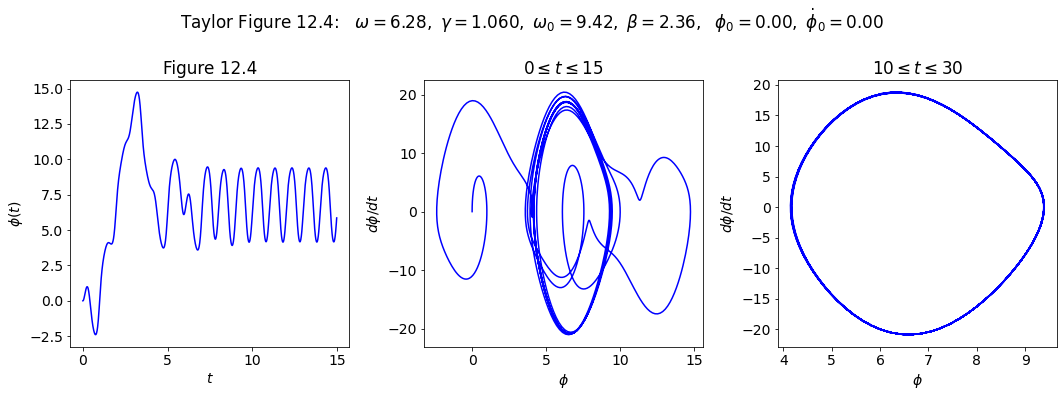
Let’s check for periodicity after the transients die out. Print out phi(t) once every period of the external driving force.
# First pass at periodicity check
start, stop = start_stop_indices(t_pts, 50., 70.)
tau_ext = 2.*np.pi / omega_ext
delta_index = int(tau_ext / delta_t)

print('   t     phi(t)')
for index in range(start, stop, delta_index):
    print(f'  {t_pts[index]:.1f}   {phi[index]:.4f}')
   t     phi(t)
  50.0   6.0366
  51.0   6.0366
  52.0   6.0366
  53.0   6.0367
  54.0   6.0366
  55.0   6.0367
  56.0   6.0366
  57.0   6.0366
  58.0   6.0366
  59.0   6.0366
  60.0   6.0366
  61.0   6.0366
  62.0   6.0366
  63.0   6.0366
  64.0   6.0366
  65.0   6.0366
  66.0   6.0366
  67.0   6.0366
  68.0   6.0366
  69.0   6.0366
Now trying the power spectrum in steady state, plotting only positive frequencies and cutting off any lower peaks from noise. We multiply the frequencies by \(2\pi\) to get the angular frequency. What do you observe?
start, stop = start_stop_indices(t_pts, 20., t_end)
signal = phi[start:stop]
power_spectrum = np.abs(np.fft.fft(signal))**2
freqs = 2.*np.pi * np.fft.fftfreq(signal.size, delta_t)
idx = np.argsort(freqs)

fig_ps = plt.figure(figsize=(5,5))
ax_ps = fig_ps.add_subplot(1,1,1)
ax_ps.semilogy(freqs[idx], power_spectrum[idx], color='blue')
ax_ps.set_xlim(0, 30.)
ax_ps.set_ylim(1.e4, 1.e9)
ax_ps.set_xlabel('frequency (Hz)')
ax_ps.set_title('Power Spectrum for Figure 12.4')

fig_ps.tight_layout()
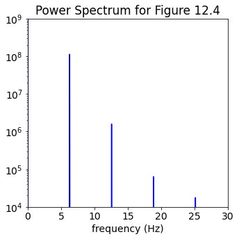
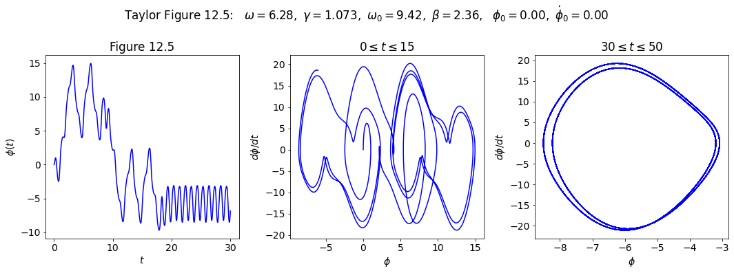
Figure 12.5: Pick conditions and then analyze#
# Labels for individual plot axes
phi_vs_time_labels = (r'$t$', r'$\phi(t)$')
phi_dot_vs_time_labels = (r'$t$', r'$d\phi/dt(t)$')
state_space_labels = (r'$\phi$', r'$d\phi/dt$')

# Common plotting time (generate the full time then use slices)
t_start = 0.
t_end = 100.
delta_t = 0.01

t_pts = np.arange(t_start, t_end+delta_t, delta_t)

# Common pendulum parameters
gamma_ext = 1.073
omega_ext = 2.*np.pi
phi_ext = 0.

omega_0 = 1.5*omega_ext
beta = omega_0/4.

# Instantiate a pendulum
p1 = Pendulum(omega_0=omega_0, beta=beta,
              gamma_ext=gamma_ext, omega_ext=omega_ext, phi_ext=phi_ext)

# calculate the driving force for t_pts
driving = p1.driving_force(t_pts)
# initial conditions specified
phi_0 = 0.
phi_dot_0 = 0.0
phi, phi_dot = p1.solve_ode(phi_0, phi_dot_0)

# Change the common font size
font_size = 14
plt.rcParams.update({'font.size': font_size})

# start the plot!
fig = plt.figure(figsize=(15,5))
overall_title = 'Taylor Figure 12.5:  ' + \
                rf' $\omega = {omega_ext:.2f},$' + \
                rf' $\gamma = {gamma_ext:.3f},$' + \
                rf' $\omega_0 = {omega_0:.2f},$' + \
                rf' $\beta = {beta:.2f},$' + \
                rf'  $\phi_0 = {phi_0:.2f},$' + \
                rf' $\dot\phi_0 = {phi_dot_0:.2f}$' + \
                '\n'     # \n means a new line (adds some space here)
fig.suptitle(overall_title, va='baseline')

# first plot: plot from t=0 to t=15
ax_a = fig.add_subplot(1,3,1)

start, stop = start_stop_indices(t_pts, 0., 30.)
plot_y_vs_x(t_pts[start : stop], phi[start : stop],
            axis_labels=phi_vs_time_labels,
            color='blue',
            label=None,
            title='Figure 12.5',
            ax=ax_a)

# second plot: state space plot from t=0 to t=15
ax_b = fig.add_subplot(1,3,2)

start, stop = start_stop_indices(t_pts, 0., 15.)
plot_y_vs_x(phi[start : stop], phi_dot[start : stop],
            axis_labels=state_space_labels,
            color='blue',
            label=None,
            title=rf'$0 \leq t \leq 15$',
            ax=ax_b)

# third plot: state space plot from t= to t=12
ax_c = fig.add_subplot(1,3,3)

start, stop = start_stop_indices(t_pts, 30., 50.)
plot_y_vs_x(phi[start : stop], phi_dot[start : stop],
            axis_labels=state_space_labels,
            color='blue',
            label=None,
            title=rf'$30 \leq t \leq 50$',
            ax=ax_c)

fig.tight_layout()
fig.savefig('Figure_12.5.png', bbox_inches='tight')  # always bbox_inches='tight'
# First pass at periodicity check
start, stop = start_stop_indices(t_pts, 50., 70.)
tau_ext = 2.*np.pi / omega_ext
delta_index = int(tau_ext / delta_t)

print('   t     phi(t)')
for index in range(start, stop, delta_index):
    print(f'  {t_pts[index]:.1f}   {phi[index]:.4f}')
   t     phi(t)
  50.0   -6.6438
  51.0   -6.4090
  52.0   -6.6438
  53.0   -6.4090
  54.0   -6.6438
  55.0   -6.4090
  56.0   -6.6439
  57.0   -6.4090
  58.0   -6.6437
  59.0   -6.4090
  60.0   -6.6438
  61.0   -6.4090
  62.0   -6.6437
  63.0   -6.4090
  64.0   -6.6438
  65.0   -6.4090
  66.0   -6.6438
  67.0   -6.4090
  68.0   -6.6438
  69.0   -6.4090
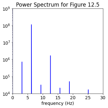
Now trying the power spectrum in steady state, plotting only positive frequencies and cutting off any lower peaks from noise. We multiply the frequencies by \(2\pi\) to get the angular frequency. What do you observe?
start, stop = start_stop_indices(t_pts, 20., t_end)
signal = phi[start:stop]
power_spectrum = np.abs(np.fft.fft(signal))**2
freqs = 2.*np.pi * np.fft.fftfreq(signal.size, delta_t)
idx = np.argsort(freqs)

fig_ps = plt.figure(figsize=(5,5))
ax_ps = fig_ps.add_subplot(1,1,1)
ax_ps.semilogy(freqs[idx], power_spectrum[idx], color='blue')
ax_ps.set_xlim(0, 30.)
ax_ps.set_ylim(1.e4, 1.e9)
ax_ps.set_xlabel('frequency (Hz)')
ax_ps.set_title('Power Spectrum for Figure 12.5')

fig_ps.tight_layout()
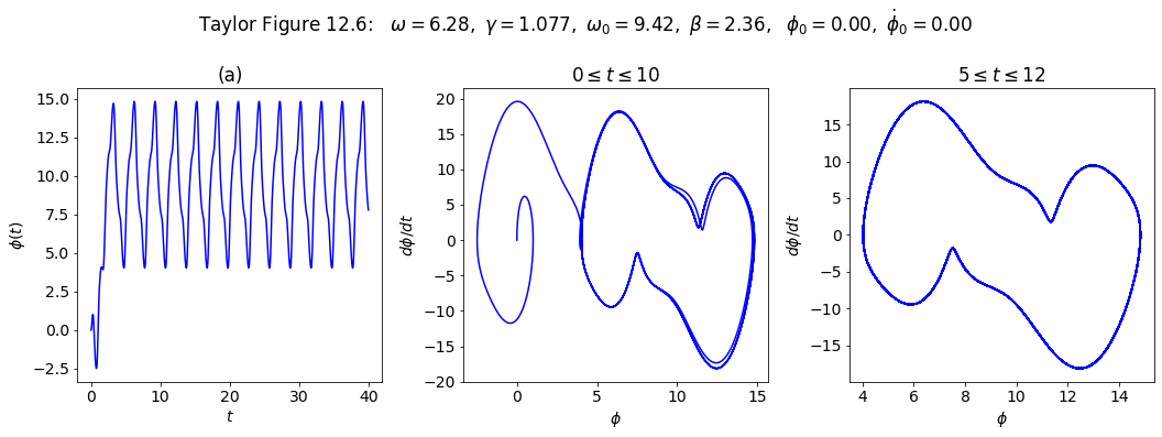
Make plots for Taylor Figure 12.6#
# Labels for individual plot axes
phi_vs_time_labels = (r'$t$', r'$\phi(t)$')
phi_dot_vs_time_labels = (r'$t$', r'$d\phi/dt(t)$')
state_space_labels = (r'$\phi$', r'$d\phi/dt$')

# Common plotting time (generate the full time then use slices)
t_start = 0.
t_end = 100.
delta_t = 0.01

t_pts = np.arange(t_start, t_end+delta_t, delta_t)

# Common pendulum parameters
gamma_ext = 1.077
omega_ext = 2.*np.pi
phi_ext = 0.

omega_0 = 1.5*omega_ext
beta = omega_0/4.

# Instantiate a pendulum
p1 = Pendulum(omega_0=omega_0, beta=beta,
              gamma_ext=gamma_ext, omega_ext=omega_ext, phi_ext=phi_ext)

# calculate the driving force for t_pts
driving = p1.driving_force(t_pts)
# initial conditions specified
phi_0 = 0.
phi_dot_0 = 0.0
phi, phi_dot = p1.solve_ode(phi_0, phi_dot_0)
phi_fig12_6 = phi

# Change the common font size
font_size = 14
plt.rcParams.update({'font.size': font_size})

# start the plot!
fig = plt.figure(figsize=(15,5))
overall_title = 'Taylor Figure 12.6:  ' + \
                rf' $\omega = {omega_ext:.2f},$' + \
                rf' $\gamma = {gamma_ext:.3f},$' + \
                rf' $\omega_0 = {omega_0:.2f},$' + \
                rf' $\beta = {beta:.2f},$' + \
                rf'  $\phi_0 = {phi_0:.2f},$' + \
                rf' $\dot\phi_0 = {phi_dot_0:.2f}$' + \
                '\n'     # \n means a new line (adds some space here)
fig.suptitle(overall_title, va='baseline')

# first plot: plot from t=0 to t=10
ax_a = fig.add_subplot(1,3,1)

start, stop = start_stop_indices(t_pts, 0., 40.)
plot_y_vs_x(t_pts[start : stop], phi[start : stop],
            axis_labels=phi_vs_time_labels,
            color='blue',
            label=None,
            title='(a)',
            ax=ax_a)

# second plot: state space plot from t=0 to t=10
ax_b = fig.add_subplot(1,3,2)

start, stop = start_stop_indices(t_pts, 0., 15.)
plot_y_vs_x(phi[start : stop], phi_dot[start : stop],
            axis_labels=state_space_labels,
            color='blue',
            label=None,
            title=rf'$0 \leq t \leq 10$',
            ax=ax_b)

# third plot: state space plot from t=5 to t=12
ax_c = fig.add_subplot(1,3,3)

start, stop = start_stop_indices(t_pts, 20, 100.)
plot_y_vs_x(phi[start : stop], phi_dot[start : stop],
            axis_labels=state_space_labels,
            color='blue',
            label=None,
            title=rf'$5 \leq t \leq 12$',
            ax=ax_c)

fig.tight_layout()
fig.savefig('Figure_12.6.png', bbox_inches='tight')  # always bbox_inches='tight'
# First pass at periodicity check
start, stop = start_stop_indices(t_pts, 50., 70.)
tau_ext = 2.*np.pi / omega_ext
delta_index = int(tau_ext / delta_t)

print('   t     phi(t)')
for index in range(start, stop, delta_index):
    print(f'  {t_pts[index]:.1f}   {phi[index]:.4f}')
   t     phi(t)
  50.0   6.8727
  51.0   13.8122
  52.0   7.7585
  53.0   6.8727
  54.0   13.8122
  55.0   7.7585
  56.0   6.8727
  57.0   13.8123
  58.0   7.7585
  59.0   6.8727
  60.0   13.8122
  61.0   7.7585
  62.0   6.8727
  63.0   13.8122
  64.0   7.7585
  65.0   6.8727
  66.0   13.8122
  67.0   7.7585
  68.0   6.8726
  69.0   13.8123
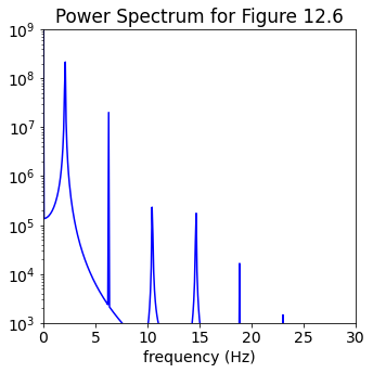
Now trying the power spectrum in steady state, plotting only positive frequencies and cutting off any lower peaks from noise. We multiply the frequencies by \(2\pi\) to get the angular frequency. What do you observe?
start, stop = start_stop_indices(t_pts, 20., t_end)
signal = phi[start:stop]
power_spectrum = np.abs(np.fft.fft(signal))**2
freqs = 2.*np.pi * np.fft.fftfreq(signal.size, delta_t)
idx = np.argsort(freqs)

fig_ps = plt.figure(figsize=(5,5))
ax_ps = fig_ps.add_subplot(1,1,1)
ax_ps.semilogy(freqs[idx], power_spectrum[idx], color='blue')
ax_ps.set_xlim(0, 30.)
ax_ps.set_ylim(1.e3, 1.e9)
ax_ps.set_xlabel('frequency (Hz)')
ax_ps.set_title('Power Spectrum for Figure 12.6')

fig_ps.tight_layout()
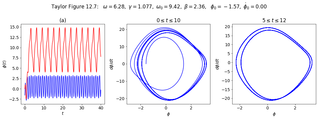
Make plots for Taylor Figure 12.7#
# Labels for individual plot axes
phi_vs_time_labels = (r'$t$', r'$\phi(t)$')
phi_dot_vs_time_labels = (r'$t$', r'$d\phi/dt(t)$')
state_space_labels = (r'$\phi$', r'$d\phi/dt$')

# Common plotting time (generate the full time then use slices)
t_start = 0.
t_end = 500.
delta_t = 0.01

t_pts = np.arange(t_start, t_end+delta_t, delta_t)

# Common pendulum parameters
gamma_ext = 1.077
omega_ext = 2.*np.pi
phi_ext = 0.

omega_0 = 1.5*omega_ext
beta = omega_0/4.

# Instantiate a pendulum
p1 = Pendulum(omega_0=omega_0, beta=beta,
              gamma_ext=gamma_ext, omega_ext=omega_ext, phi_ext=phi_ext)

# calculate the driving force for t_pts
driving = p1.driving_force(t_pts)
# initial conditions specified
phi_0 = -np.pi/2.
phi_dot_0 = 0.0
phi, phi_dot = p1.solve_ode(phi_0, phi_dot_0)

# Change the common font size
font_size = 14
plt.rcParams.update({'font.size': font_size})

# start the plot!
fig = plt.figure(figsize=(15,5))
overall_title = 'Taylor Figure 12.7:  ' + \
                rf' $\omega = {omega_ext:.2f},$' + \
                rf' $\gamma = {gamma_ext:.3f},$' + \
                rf' $\omega_0 = {omega_0:.2f},$' + \
                rf' $\beta = {beta:.2f},$' + \
                rf'  $\phi_0 = {phi_0:.2f},$' + \
                rf' $\dot\phi_0 = {phi_dot_0:.2f}$' + \
                '\n'     # \n means a new line (adds some space here)
fig.suptitle(overall_title, va='baseline')

# first plot: plot from t=0 to t=10
ax_a = fig.add_subplot(1,3,1)

start, stop = start_stop_indices(t_pts, 0., 40.)
plot_y_vs_x(t_pts[start : stop], phi[start : stop],
            axis_labels=phi_vs_time_labels,
            color='blue',
            label=None,
            title='(a)',
            ax=ax_a)
plot_y_vs_x(t_pts[start : stop], phi_fig12_6[start : stop],
            axis_labels=phi_vs_time_labels,
            color='red',
            label=None,
            ax=ax_a)

# second plot: state space plot from t=0 to t=15
ax_b = fig.add_subplot(1,3,2)

start, stop = start_stop_indices(t_pts, 0., 15.)
plot_y_vs_x(phi[start : stop], phi_dot[start : stop],
            axis_labels=state_space_labels,
            color='blue',
            label=None,
            title=rf'$0 \leq t \leq 10$',
            ax=ax_b)

# third plot: state space plot from t=5 to t=12
ax_c = fig.add_subplot(1,3,3)

start, stop = start_stop_indices(t_pts, 20, 100.)
plot_y_vs_x(phi[start : stop], phi_dot[start : stop],
            axis_labels=state_space_labels,
            color='blue',
            label=None,
            title=rf'$5 \leq t \leq 12$',
            ax=ax_c)

fig.tight_layout()
fig.savefig('Figure_12.7.png', bbox_inches='tight')  # always bbox_inches='tight'
# First pass at periodicity check
start, stop = start_stop_indices(t_pts, 50., 70.)
tau_ext = 2.*np.pi / omega_ext
delta_index = int(tau_ext / delta_t)

print('   t     phi(t)')
for index in range(start, stop, delta_index):
    print(f'  {t_pts[index]:.1f}   {phi[index]:.4f}')
   t     phi(t)
  50.0   -0.1071
  51.0   -0.4051
  52.0   -0.1071
  53.0   -0.4050
  54.0   -0.1071
  55.0   -0.4050
  56.0   -0.1071
  57.0   -0.4050
  58.0   -0.1071
  59.0   -0.4051
  60.0   -0.1071
  61.0   -0.4049
  62.0   -0.1070
  63.0   -0.4051
  64.0   -0.1071
  65.0   -0.4050
  66.0   -0.1071
  67.0   -0.4050
  68.0   -0.1071
  69.0   -0.4050
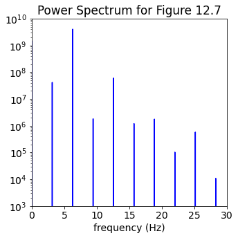
Now trying the power spectrum in steady state, plotting only positive frequencies and cutting off any lower peaks from noise. We multiply the frequencies by \(2\pi\) to get the angular frequency. What do you observe?
start, stop = start_stop_indices(t_pts, 20., t_end)
signal = phi[start:stop]
power_spectrum = np.abs(np.fft.fft(signal))**2
freqs = 2.*np.pi * np.fft.fftfreq(signal.size, delta_t)
idx = np.argsort(freqs)

fig_ps = plt.figure(figsize=(5,5))
ax_ps = fig_ps.add_subplot(1,1,1)
ax_ps.semilogy(freqs[idx], power_spectrum[idx], color='blue')
ax_ps.set_xlim(0, 30.)
ax_ps.set_ylim(1.e3, 1.e10)
ax_ps.set_xlabel('frequency (Hz)')
ax_ps.set_title('Power Spectrum for Figure 12.7')

fig_ps.tight_layout()
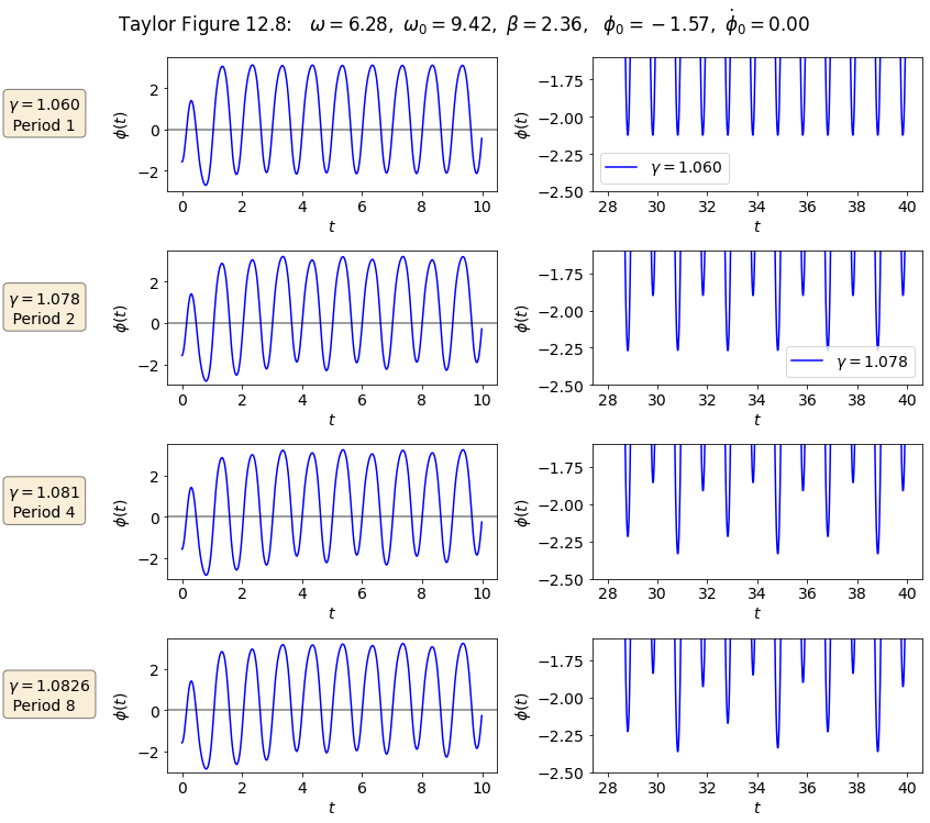
Make plots for Taylor Figure 12.8#
Now we try to plot a period doubling cascade as in Figure 12.8. This will mean plots of four different conditions, each with two plots.
# Labels for individual plot axes
phi_vs_time_labels = (r'$t$', r'$\phi(t)$')
phi_dot_vs_time_labels = (r'$t$', r'$d\phi/dt(t)$')
state_space_labels = (r'$\phi$', r'$d\phi/dt$')

# Common plotting time (generate the full time then use slices)
t_start = 0.
t_end = 100.
delta_t = 0.01

t_pts = np.arange(t_start, t_end+delta_t, delta_t)

# Common parameters
omega_ext = 2.*np.pi
phi_ext = 0.

omega_0 = 1.5*omega_ext
beta = omega_0/4.

# Instantiate the pendulu s
gamma_ext = 1.060
p1 = Pendulum(omega_0=omega_0, beta=beta,
              gamma_ext=gamma_ext, omega_ext=omega_ext, phi_ext=phi_ext)

gamma_ext = 1.078
p2 = Pendulum(omega_0=omega_0, beta=beta,
              gamma_ext=gamma_ext, omega_ext=omega_ext, phi_ext=phi_ext)

gamma_ext = 1.081
p3 = Pendulum(omega_0=omega_0, beta=beta,
              gamma_ext=gamma_ext, omega_ext=omega_ext, phi_ext=phi_ext)

gamma_ext = 1.0826
p4 = Pendulum(omega_0=omega_0, beta=beta,
              gamma_ext=gamma_ext, omega_ext=omega_ext, phi_ext=phi_ext)

# calculate the driving force for t_pts (all the same)
driving = p1.driving_force(t_pts)
# same initial conditions specified
phi_0 = -np.pi / 2.
phi_dot_0 = 0.

# solve each of the pendulum odes
phi_1, phi_dot_1 = p1.solve_ode(phi_0, phi_dot_0)
phi_2, phi_dot_2 = p2.solve_ode(phi_0, phi_dot_0)
phi_3, phi_dot_3 = p3.solve_ode(phi_0, phi_dot_0)
phi_4, phi_dot_4 = p4.solve_ode(phi_0, phi_dot_0)

# Change the common font size
font_size = 14
plt.rcParams.update({'font.size': font_size})
box_props = dict(boxstyle='round', facecolor='wheat', alpha=0.5)

# start the plot!
fig = plt.figure(figsize=(12,10))
overall_title = 'Taylor Figure 12.8:  ' + \
                rf' $\omega = {omega_ext:.2f},$' + \
                rf' $\omega_0 = {omega_0:.2f},$' + \
                rf' $\beta = {beta:.2f},$' + \
                rf'  $\phi_0 = {phi_0:.2f},$' + \
                rf' $\dot\phi_0 = {phi_dot_0:.2f}$' + \
                '\n'     # \n means a new line (adds some space here)
fig.suptitle(overall_title, va='baseline')

# plot 1a: plot from t=0 to t=10
ax_1a = fig.add_subplot(4,2,1)
start, stop = start_stop_indices(t_pts, 0., 10.)
plot_y_vs_x(t_pts[start : stop], phi_1[start : stop],
            axis_labels=phi_vs_time_labels,
            color='blue',
            label=None,
            ax=ax_1a)
ax_1a.set_ylim(-3, 3.5)
ax_1a.axhline(y=0., color='black', alpha=0.5)
textstr = r'$\gamma = 1.060$' + '\n' + r' Period 1'
ax_1a.text(-5.8, 0., textstr, bbox=box_props)

# plot 1b: plot from t=28 to t=40 blown up
ax_1b = fig.add_subplot(4,2,2)
start, stop = start_stop_indices(t_pts, 28., 40.)
plot_y_vs_x(t_pts[start : stop], phi_1[start : stop],
            axis_labels=phi_vs_time_labels,
            color='blue',
            label=rf'$\gamma = 1.060$',
            ax=ax_1b)
ax_1b.set_ylim(-2.5, -1.6)

# plot 2a: plot from t=0 to t=10
ax_2a = fig.add_subplot(4,2,3)
start, stop = start_stop_indices(t_pts, 0., 10.)
plot_y_vs_x(t_pts[start : stop], phi_2[start : stop],
            axis_labels=phi_vs_time_labels,
            color='blue',
            label=None,
            ax=ax_2a)
ax_2a.set_ylim(-3, 3.5)
ax_2a.axhline(y=0., color='black', alpha=0.5)
textstr = r'$\gamma = 1.078$' + '\n' + r' Period 2'
ax_2a.text(-5.8, 0., textstr, bbox=box_props)

# plot 2b: plot from t=28 to t=40 blown up
ax_2b = fig.add_subplot(4,2,4)
start, stop = start_stop_indices(t_pts, 28., 40.)
plot_y_vs_x(t_pts[start : stop], phi_2[start : stop],
            axis_labels=phi_vs_time_labels,
            color='blue',
            label=rf'$\gamma = 1.078$',
            ax=ax_2b)
ax_2b.set_ylim(-2.5, -1.6)

# plot 3a: plot from t=0 to t=10
ax_3a = fig.add_subplot(4,2,5)
start, stop = start_stop_indices(t_pts, 0., 10.)
plot_y_vs_x(t_pts[start : stop], phi_3[start : stop],
            axis_labels=phi_vs_time_labels,
            color='blue',
            label=None,
            ax=ax_3a)
ax_3a.set_ylim(-3, 3.5)
ax_3a.axhline(y=0., color='black', alpha=0.5)
textstr = r'$\gamma = 1.081$' + '\n' + r' Period 4'
ax_3a.text(-5.8, 0., textstr, bbox=box_props)

# plot 3b: plot from t=28 to t=40 blown up
ax_3b = fig.add_subplot(4,2,6)
start, stop = start_stop_indices(t_pts, 28., 40.)
plot_y_vs_x(t_pts[start : stop], phi_3[start : stop],
            axis_labels=phi_vs_time_labels,
            color='blue',
            label=None,
            ax=ax_3b)
ax_3b.set_ylim(-2.5, -1.6)

# plot 4a: plot from t=0 to t=10
ax_4a = fig.add_subplot(4,2,7)
start, stop = start_stop_indices(t_pts, 0., 10.)
plot_y_vs_x(t_pts[start : stop], phi_4[start : stop],
            axis_labels=phi_vs_time_labels,
            color='blue',
            label=None,
            ax=ax_4a)
ax_4a.set_ylim(-3, 3.5)
ax_4a.axhline(y=0., color='black', alpha=0.5)
textstr = r'$\gamma = 1.0826$' + '\n' + r' Period 8'
ax_4a.text(-5.8, 0., textstr, bbox=box_props)

# plot 4b: plot from t=28 to t=40 blown up
ax_4b = fig.add_subplot(4,2,8)
start, stop = start_stop_indices(t_pts, 28., 40.)
plot_y_vs_x(t_pts[start : stop], phi_4[start : stop],
            axis_labels=phi_vs_time_labels,
            color='blue',
            label=None,
            ax=ax_4b)
ax_4b.set_ylim(-2.5, -1.6)

fig.tight_layout()
fig.savefig('Figure_12.8.png', bbox_inches='tight')  # always bbox_inches='tight'