Multiple pendulum plots. Section 12.5: Chaos and sensitivity to initial conditions
Contents
Multiple pendulum plots. Section 12.5: Chaos and sensitivity to initial conditions#
Use Pendulum class to generate basic pendulum plots. Applied here to figures from Taylor Section 12.5.
Last revised 26-Jan-2019 by Dick Furnstahl (furnstahl.1@osu.edu).
%matplotlib inline
import numpy as np
from scipy.integrate import odeint

import matplotlib.pyplot as plt
Pendulum class and utility functions#
class Pendulum():
    """
    Pendulum class implements the parameters and differential equation for
     a pendulum using the notation from Taylor.

    Parameters
    ----------
    omega_0 : float
        natural frequency of the pendulum (\sqrt{g/l} where l is the
        pendulum length)
    beta : float
        coefficient of friction
    gamma_ext : float
        amplitude of external force is gamma * omega_0**2
    omega_ext : float
        frequency of external force
    phi_ext : float
        phase angle for external force

    Methods
    -------
    dy_dt(y, t)
        Returns the right side of the differential equation in vector y,
        given time t and the corresponding value of y.
    driving_force(t)
        Returns the value of the external driving force at time t.
    """
    def __init__(self, omega_0=1., beta=0.2,
                 gamma_ext=0.2, omega_ext=0.689, phi_ext=0.
                ):
        self.omega_0 = omega_0
        self.beta = beta
        self.gamma_ext = gamma_ext
        self.omega_ext = omega_ext
        self.phi_ext = phi_ext

    def dy_dt(self, y, t):
        """
        This function returns the right-hand side of the diffeq:
        [dphi/dt d^2phi/dt^2]

        Parameters
        ----------
        y : float
            A 2-component vector with y[0] = phi(t) and y[1] = dphi/dt
        t : float
            time

        Returns
        -------

        """
        F_ext = self.driving_force(t)
        return [y[1], -self.omega_0**2 * np.sin(y[0]) - 2.*self.beta * y[1] \
                       + F_ext]

    def driving_force(self, t):
        """
        This function returns the value of the driving force at time t.
        """
        return self.gamma_ext * self.omega_0**2 \
                              * np.cos(self.omega_ext*t + self.phi_ext)

    def solve_ode(self, phi_0, phi_dot_0, abserr=1.0e-8, relerr=1.0e-6):
        """
        Solve the ODE given initial conditions.
        For now use odeint, but we have the option to switch.
        Specify smaller abserr and relerr to get more precision.
        """
        y = [phi_0, phi_dot_0]
        phi, phi_dot = odeint(self.dy_dt, y, t_pts,
                              atol=abserr, rtol=relerr).T
        return phi, phi_dot
def plot_y_vs_x(x, y, axis_labels=None, label=None, title=None,
                color=None, linestyle=None, semilogy=False, loglog=False,
                ax=None):
    """
    Generic plotting function: return a figure axis with a plot of y vs. x,
    with line color and style, title, axis labels, and line label
    """
    if ax is None:        # if the axis object doesn't exist, make one
        ax = plt.gca()

    if (semilogy):
        line, = ax.semilogy(x, y, label=label,
                            color=color, linestyle=linestyle)
    elif (loglog):
        line, = ax.loglog(x, y, label=label,
                          color=color, linestyle=linestyle)
    else:
        line, = ax.plot(x, y, label=label,
                    color=color, linestyle=linestyle)

    if label is not None:    # if a label if passed, show the legend
        ax.legend()
    if title is not None:    # set a title if one if passed
        ax.set_title(title)
    if axis_labels is not None:  # set x-axis and y-axis labels if passed
        ax.set_xlabel(axis_labels[0])
        ax.set_ylabel(axis_labels[1])

    return ax, line
def start_stop_indices(t_pts, plot_start, plot_stop):
    """Given an array (e.g., of times) and desired starting and stop values,
        return the array indices that are closest to those values.
    """
    start_index = (np.fabs(t_pts-plot_start)).argmin()  # index in t_pts array
    stop_index = (np.fabs(t_pts-plot_stop)).argmin()  # index in t_pts array
    return start_index, stop_index
Make plots for Taylor Figure 12.10#
We’ll set it up with the specified parameters.
# Labels for individual plot axes
phi_vs_time_labels = (r'$t$', r'$\phi(t)$')
phi_dot_vs_time_labels = (r'$t$', r'$d\phi/dt(t)$')
state_space_labels = (r'$\phi$', r'$d\phi/dt$')

# Common plotting time (generate the full time then use slices)
t_start = 0.
t_end = 1000.
delta_t = 0.01

t_pts = np.arange(t_start, t_end+delta_t, delta_t)

# Common pendulum parameters
gamma_ext = 1.105
omega_ext = 2.*np.pi
phi_ext = 0.

omega_0 = 1.5*omega_ext
beta = omega_0/4.

# Instantiate a pendulum
p1 = Pendulum(omega_0=omega_0, beta=beta,
              gamma_ext=gamma_ext, omega_ext=omega_ext, phi_ext=phi_ext)

# calculate the driving force for t_pts
driving = p1.driving_force(t_pts)
# initial conditions specified
phi_0 = -np.pi / 2.
phi_dot_0 = 0.0
phi, phi_dot = p1.solve_ode(phi_0, phi_dot_0)

# Change the common font size
font_size = 14
plt.rcParams.update({'font.size': font_size})

# start the plot!
fig = plt.figure(figsize=(15,5))
overall_title = 'Taylor Figure 12.10:  ' + \
                rf' $\omega = {omega_ext:.2f},$' + \
                rf' $\gamma = {gamma_ext:.3f},$' + \
                rf' $\omega_0 = {omega_0:.2f},$' + \
                rf' $\beta = {beta:.2f},$' + \
                rf'  $\phi_0 = {phi_0:.2f},$' + \
                rf' $\dot\phi_0 = {phi_dot_0:.2f}$' + \
                '\n'     # \n means a new line (adds some space here)
fig.suptitle(overall_title, va='baseline')

# first plot: plot from t=0 to t=15
ax_a = fig.add_subplot(1,3,1)

start, stop = start_stop_indices(t_pts, 0., 30.)
plot_y_vs_x(t_pts[start : stop], phi[start : stop],
            axis_labels=phi_vs_time_labels,
            color='blue',
            label=None,
            title='Figure 12.4',
            ax=ax_a)

# second plot: state space plot from t=0 to t=15
ax_b = fig.add_subplot(1,3,2)

start, stop = start_stop_indices(t_pts, 0., 15.)
plot_y_vs_x(phi[start : stop], phi_dot[start : stop],
            axis_labels=state_space_labels,
            color='blue',
            label=None,
            title=rf'$0 \leq t \leq 15$',
            ax=ax_b)

# third plot: state space plot from t= to t=12
ax_c = fig.add_subplot(1,3,3)

start, stop = start_stop_indices(t_pts, 10., 30.)
plot_y_vs_x(phi[start : stop], phi_dot[start : stop],
            axis_labels=state_space_labels,
            color='blue',
            label=None,
            title=rf'$10 \leq t \leq 30$',
            ax=ax_c)

fig.tight_layout()
fig.savefig('Figure_12.10.png', bbox_inches='tight')  # always bbox_inches='tight'
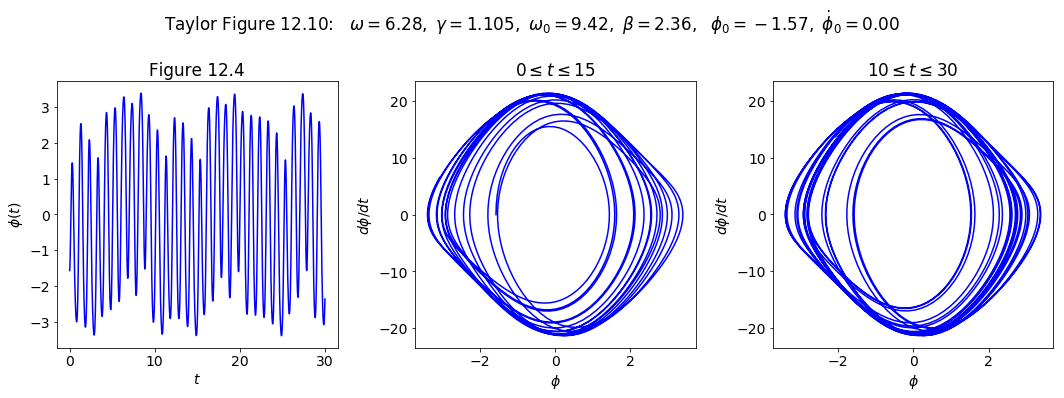
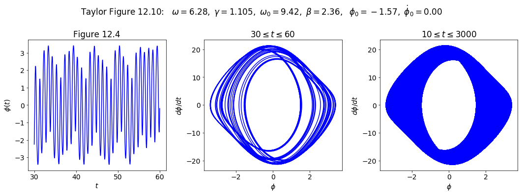
Maybe we just didn’t wait long enough! Let’s try t from 30 to 60 instead:
# initial conditions specified
phi_0 = -np.pi / 2.
phi_dot_0 = 0.0
phi, phi_dot = p1.solve_ode(phi_0, phi_dot_0)

# Change the common font size
font_size = 14
plt.rcParams.update({'font.size': font_size})

# start the plot!
fig = plt.figure(figsize=(15,5))
overall_title = 'Taylor Figure 12.10:  ' + \
                rf' $\omega = {omega_ext:.2f},$' + \
                rf' $\gamma = {gamma_ext:.3f},$' + \
                rf' $\omega_0 = {omega_0:.2f},$' + \
                rf' $\beta = {beta:.2f},$' + \
                rf'  $\phi_0 = {phi_0:.2f},$' + \
                rf' $\dot\phi_0 = {phi_dot_0:.2f}$' + \
                '\n'     # \n means a new line (adds some space here)
fig.suptitle(overall_title, va='baseline')

# first plot: plot from t=0 to t=15
ax_a = fig.add_subplot(1,3,1)

start, stop = start_stop_indices(t_pts, 30., 60.)
plot_y_vs_x(t_pts[start : stop], phi[start : stop],
            axis_labels=phi_vs_time_labels,
            color='blue',
            label=None,
            title='Figure 12.4',
            ax=ax_a)

# second plot: state space plot from t=0 to t=15
ax_b = fig.add_subplot(1,3,2)

start, stop = start_stop_indices(t_pts, 30., 60.)
plot_y_vs_x(phi[start : stop], phi_dot[start : stop],
            axis_labels=state_space_labels,
            color='blue',
            label=None,
            title=rf'$30 \leq t \leq 60$',
            ax=ax_b)

# third plot: state space plot from t= to t=12
ax_c = fig.add_subplot(1,3,3)

start, stop = start_stop_indices(t_pts, 10., 1000.)
plot_y_vs_x(phi[start : stop], phi_dot[start : stop],
            axis_labels=state_space_labels,
            color='blue',
            label=None,
            title=rf'$10 \leq t \leq 1000$',
            ax=ax_c)

fig.tight_layout()
fig.savefig('Figure_12.10.png', bbox_inches='tight')  # always bbox_inches='tight'

Let’s check for periodicity after the transients die out. Print out phi(t) once every period of the external driving force.
# First pass at periodicity check
start, stop = start_stop_indices(t_pts, 50., 70.)
tau_ext = 2.*np.pi / omega_ext
delta_index = int(tau_ext / delta_t)

print('   t     phi(t)')
for index in range(start, stop, delta_index):
    print(f'  {t_pts[index]:.1f}   {phi[index]:.4f}')
   t     phi(t)
  50.0   -0.2803
  51.0   -0.0342
  52.0   -2.1546
  53.0   -2.9949
  54.0   -1.2143
  55.0   -0.6228
  56.0   -0.0495
  57.0   -0.7050
  58.0   -0.0835
  59.0   -0.2642
  60.0   -0.0338
  61.0   -1.8846
  62.0   -2.6286
  63.0   -2.6078
  64.0   -2.6660
  65.0   -2.5192
  66.0   -2.8383
  67.0   -1.9275
  68.0   -2.6460
  69.0   -2.5636
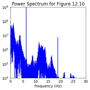
Now trying the power spectrum in steady state, plotting only positive frequencies and cutting off any lower peaks from noise. We multiply the frequencies by \(2\pi\) to get the angular frequency. What do you observe?
start, stop = start_stop_indices(t_pts, 20., t_end)
signal = phi[start:stop]
power_spectrum = np.abs(np.fft.fft(signal))**2
freqs = 2.*np.pi * np.fft.fftfreq(signal.size, delta_t)
idx = np.argsort(freqs)

fig_ps = plt.figure(figsize=(5,5))
ax_ps = fig_ps.add_subplot(1,1,1)
ax_ps.semilogy(freqs[idx], power_spectrum[idx], color='blue')
ax_ps.set_xlim(0, 30.)
ax_ps.set_ylim(1.e4, 1.e9)
ax_ps.set_xlabel('frequency (Hz)')
ax_ps.set_title('Power Spectrum for Figure 12.10')

fig_ps.tight_layout()
# Labels for individual plot axes
phi_vs_time_labels = (r'$t$', r'$\phi(t)$')
phi_dot_vs_time_labels = (r'$t$', r'$d\phi/dt(t)$')
state_space_labels = (r'$\phi$', r'$d\phi/dt$')

# Common plotting time (generate the full time then use slices)
t_start = 0.
t_end = 3000.
delta_t = 0.01

t_pts = np.arange(t_start, t_end+delta_t, delta_t)

# Common pendulum parameters
gamma_ext = 1.105
omega_ext = 2.*np.pi
phi_ext = 0.

omega_0 = 1.5*omega_ext
beta = omega_0/4.

# Instantiate a pendulum
p1 = Pendulum(omega_0=omega_0, beta=beta,
              gamma_ext=gamma_ext, omega_ext=omega_ext, phi_ext=phi_ext)

# calculate the driving force for t_pts
driving = p1.driving_force(t_pts)
# initial conditions specified
phi_0 = -np.pi / 2.
phi_dot_0 = 0.0
phi, phi_dot = p1.solve_ode(phi_0, phi_dot_0)

# Change the common font size
font_size = 14
plt.rcParams.update({'font.size': font_size})

# start the plot!
fig = plt.figure(figsize=(15,5))
overall_title = 'Taylor Figure 12.10:  ' + \
                rf' $\omega = {omega_ext:.2f},$' + \
                rf' $\gamma = {gamma_ext:.3f},$' + \
                rf' $\omega_0 = {omega_0:.2f},$' + \
                rf' $\beta = {beta:.2f},$' + \
                rf'  $\phi_0 = {phi_0:.2f},$' + \
                rf' $\dot\phi_0 = {phi_dot_0:.2f}$' + \
                '\n'     # \n means a new line (adds some space here)
fig.suptitle(overall_title, va='baseline')

# first plot: plot from t=0 to t=15
ax_a = fig.add_subplot(1,3,1)

start, stop = start_stop_indices(t_pts, 30., 60.)
plot_y_vs_x(t_pts[start : stop], phi[start : stop],
            axis_labels=phi_vs_time_labels,
            color='blue',
            label=None,
            title='Figure 12.4',
            ax=ax_a)

# second plot: state space plot from t=0 to t=15
ax_b = fig.add_subplot(1,3,2)

start, stop = start_stop_indices(t_pts, 30., 60.)
plot_y_vs_x(phi[start : stop], phi_dot[start : stop],
            axis_labels=state_space_labels,
            color='blue',
            label=None,
            title=rf'$30 \leq t \leq 60$',
            ax=ax_b)

# third plot: state space plot from t= to t=12
ax_c = fig.add_subplot(1,3,3)

start, stop = start_stop_indices(t_pts, 10., 3000.)
plot_y_vs_x(phi[start : stop], phi_dot[start : stop],
            axis_labels=state_space_labels,
            color='blue',
            label=None,
            title=rf'$10 \leq t \leq 3000$',
            ax=ax_c)

fig.tight_layout()
fig.savefig('Figure_12.10.png', bbox_inches='tight')  # always bbox_inches='tight'
Make plots for Taylor figure 12.11 in section 12.5#
This time we plot \(\Delta \phi\).
# Labels for individual plot axes
phi_vs_time_labels = (r'$t$', r'$\phi(t)$')
Delta_phi_vs_time_labels = (r'$t$', r'$\Delta\phi(t)$')
phi_dot_vs_time_labels = (r'$t$', r'$d\phi/dt(t)$')
state_space_labels = (r'$\phi$', r'$d\phi/dt$')

# Common plotting time (generate the full time then use slices)
t_start = 0.
t_end = 100.
delta_t = 0.01

t_pts = np.arange(t_start, t_end+delta_t, delta_t)

# Common pendulum parameters
gamma_ext = 0.1
omega_ext = 2.*np.pi
phi_ext = 0.

omega_0 = 1.5*omega_ext
beta = omega_0/4.

# Instantiate a pendulum
p1 = Pendulum(omega_0=omega_0, beta=beta,
              gamma_ext=gamma_ext, omega_ext=omega_ext, phi_ext=phi_ext)

# calculate the driving force for t_pts
driving = p1.driving_force(t_pts)
# make a plot of Delta phi for same pendulum but two different initial conds
phi_0_1 = -np.pi / 2.
phi_dot_0 = 0.0
phi_1, phi_dot_1 = p1.solve_ode(phi_0_1, phi_dot_0)

phi_0_2 = phi_0_1 - .1   # .1 radian lower
phi_dot_0 = 0.0
phi_2, phi_dot_2 = p1.solve_ode(phi_0_2, phi_dot_0)

# Calculate the absolute value of \phi_2 - \phi_1
Delta_phi = np.fabs(phi_2 - phi_1)

# Change the common font size
font_size = 14
plt.rcParams.update({'font.size': font_size})

# start the plot!
fig = plt.figure(figsize=(10,10))
overall_title = 'Taylor figure 12.11:  ' + \
                rf' $\omega = {omega_ext:.2f},$' + \
                rf' $\gamma = {gamma_ext:.3f},$' + \
                rf' $\omega_0 = {omega_0:.2f},$' + \
                rf' $\beta = {beta:.2f}$' + \
                '\n'     # \n means a new line (adds some space here)
fig.suptitle(overall_title, va='baseline')

# two plot: plot from t=0 to t=8 and another from t=0 to t=100
ax_a = fig.add_subplot(2,1,1)

start, stop = start_stop_indices(t_pts, 0., 10.)
ax_a.semilogy(t_pts[start : stop], Delta_phi[start : stop],
            color='blue', label=None)
ax_a.set_xlabel('t')
ax_a.set_ylabel(r'$|\Delta\phi|$')

ax_b = fig.add_subplot(2,1,2)

start, stop = start_stop_indices(t_pts, 0., 100.)
plot_y_vs_x(t_pts[start : stop], Delta_phi[start : stop],
            color='blue', label=None, semilogy=True)
ax_b.set_xlabel('t')
ax_b.set_ylabel(r'$|\Delta\phi|$')

fig.tight_layout()
# always bbox_inches='tight' for best results.  Further adjustments also.
fig.savefig('figure_12.11.png', bbox_inches='tight')
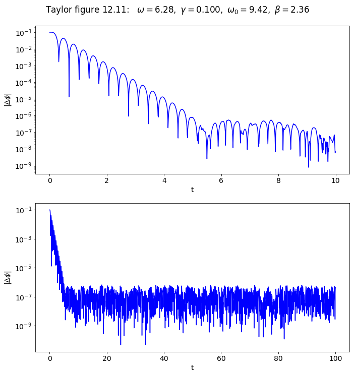
What is setting the limit here? Here it “real” or a numerical artifact?
Repeat but change abserr and relerr to 1.e-10, which is \(1.0 \times 10^{-10}\).
# make a plot of Delta phi for same pendulum but two different initial conds
phi_0_1 = phi_0 = -np.pi / 2.
phi_dot_0 = 0.0
phi_1, phi_dot_1 = p1.solve_ode(phi_0_1, phi_dot_0,
                                abserr=1.e-10, relerr=1.e-10)

phi_0_2 = phi_0_1 - .1   # .1 radian lower
phi_dot_0 = 0.0
phi_2, phi_dot_2 = p1.solve_ode(phi_0_2, phi_dot_0,
                                abserr=1.e-10, relerr=1.e-10)

# Calculate the absolute value of \phi_2 - \phi_1
Delta_phi = np.fabs(phi_2 - phi_1)

# Change the common font size
font_size = 14
plt.rcParams.update({'font.size': font_size})

# start the plot!
fig = plt.figure(figsize=(10,10))
overall_title = 'Taylor figure 12.11:  ' + \
                rf' $\omega = {omega_ext:.2f},$' + \
                rf' $\gamma = {gamma_ext:.3f},$' + \
                rf' $\omega_0 = {omega_0:.2f},$' + \
                rf' $\beta = {beta:.2f}$' + \
                '\n'     # \n means a new line (adds some space here)
fig.suptitle(overall_title, va='baseline')

# two plot: plot from t=0 to t=8 and another from t=0 to t=100
ax_a = fig.add_subplot(2,1,1)

start, stop = start_stop_indices(t_pts, 0., 10.)
ax_a.semilogy(t_pts[start : stop], Delta_phi[start : stop],
            color='blue', label=None)
ax_a.set_xlabel('t')
ax_a.set_ylabel(r'$|\Delta\phi|$')

ax_b = fig.add_subplot(2,1,2)

start, stop = start_stop_indices(t_pts, 0., 100.)
plot_y_vs_x(t_pts[start : stop], Delta_phi[start : stop],
            color='blue', label=None, semilogy=True)
ax_b.set_xlabel('t')
ax_b.set_ylabel(r'$|\Delta\phi|$')

fig.tight_layout()
# always bbox_inches='tight' for best results.  Further adjustments also.
fig.savefig('figure_12.11.png', bbox_inches='tight')
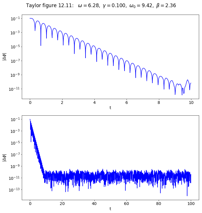
Ok, now we see the expect exponential decay from the linear regime:
\(\begin{align} \Delta\phi(t) = D e^{-\beta t} \cos(\omega_1 t - \delta) \end{align}\)
which implies an exponential decay times an oscillating term, meaning we get something like the graph!
Does the slope work out? We see that \(\log_{10}\Delta\phi\) vs. \(t\) is a straight line. But
\(\begin{align} \log_{10}[\Delta\phi(t)] = \log_{10}D - \beta t \log_{10}e + \log_{10} \cos(\omega_1 t - \delta) \end{align}\)
so on a semi-log plot, the slope is \(-\beta\log_{10} e\). At \(t\) goes from 0 to 10, \(\log_{10}[\Delta\phi(t)]\) goes from \(-1\) to \(-11\), so the slope is about \(-1\). Therefore, this predicts \(\beta \approx 1/ \log_{10} e\). Check it out:
1./np.log10(np.e)
2.302585092994046
Yep, it works! Let’s check the state space plots together:
fig_ss = plt.figure(figsize=(12,6))

ax_ss1 = fig_ss.add_subplot(1,2,1)
start, stop = start_stop_indices(t_pts, 0., 32)
plot_y_vs_x(phi_1[start : stop], phi_dot_1[start : stop],
            axis_labels=state_space_labels,
            color='blue',
            label=None,
            title=rf'$0 \leq t \leq 32$',
            ax=ax_ss1)
plot_y_vs_x(phi_2[start : stop], phi_dot_2[start : stop],
            axis_labels=state_space_labels,
            color='red',
            label=None,
            title=None,
            ax=ax_ss1)

# now skip the transients
ax_ss2 = fig_ss.add_subplot(1,2,2)
start, stop = start_stop_indices(t_pts, 10., 32)
plot_y_vs_x(phi_1[start : stop], phi_dot_1[start : stop],
            axis_labels=state_space_labels,
            color='blue',
            label=None,
            title=rf'$10 \leq t \leq 32$',
            ax=ax_ss2)
plot_y_vs_x(phi_2[start : stop], phi_dot_2[start : stop],
            axis_labels=state_space_labels,
            color='red',
            label=None,
            title=None,
            ax=ax_ss2)

fig_ss.tight_layout()

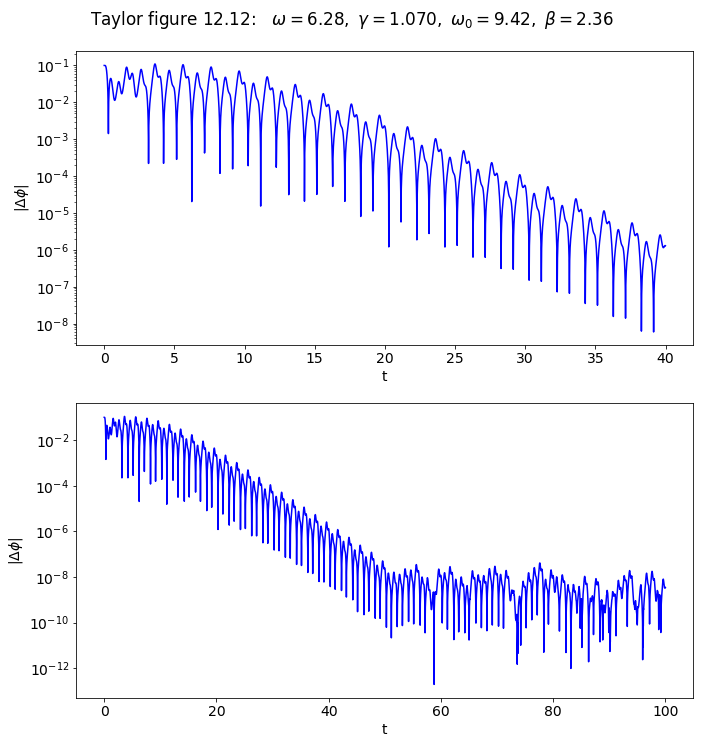
Make plots for Taylor figure 12.12: Looking at \(\Delta\phi\) for \(\gamma = 1.07\)#
# Labels for individual plot axes
phi_vs_time_labels = (r'$t$', r'$\phi(t)$')
Delta_phi_vs_time_labels = (r'$t$', r'$\Delta\phi(t)$')
phi_dot_vs_time_labels = (r'$t$', r'$d\phi/dt(t)$')
state_space_labels = (r'$\phi$', r'$d\phi/dt$')

# Common plotting time (generate the full time then use slices)
t_start = 0.
t_end = 100.
delta_t = 0.01

t_pts = np.arange(t_start, t_end+delta_t, delta_t)

# Common pendulum parameters
gamma_ext = 1.07
omega_ext = 2.*np.pi
phi_ext = 0.

omega_0 = 1.5*omega_ext
beta = omega_0/4.

# Instantiate a pendulum
p1 = Pendulum(omega_0=omega_0, beta=beta,
              gamma_ext=gamma_ext, omega_ext=omega_ext, phi_ext=phi_ext)

# calculate the driving force for t_pts
driving = p1.driving_force(t_pts)
Set abserr and relerr to 1.e-10 from the beginning.
# make a plot of Delta phi for same pendulum but two different initial conds
phi_0_1 = -np.pi / 2.
phi_dot_0 = 0.0
phi_1, phi_dot_1 = p1.solve_ode(phi_0_1, phi_dot_0,
                                abserr=1.e-10, relerr=1.e-10)

phi_0_2 = phi_0_1 - .1   # .1 radian lower
phi_dot_0 = 0.0
phi_2, phi_dot_2 = p1.solve_ode(phi_0_2, phi_dot_0,
                                abserr=1.e-10, relerr=1.e-10)

# Calculate the absolute value of \phi_2 - \phi_1
Delta_phi = np.fabs(phi_2 - phi_1)

# Change the common font size
font_size = 14
plt.rcParams.update({'font.size': font_size})

# start the plot!
fig = plt.figure(figsize=(10,10))
overall_title = 'Taylor figure 12.12:  ' + \
                rf' $\omega = {omega_ext:.2f},$' + \
                rf' $\gamma = {gamma_ext:.3f},$' + \
                rf' $\omega_0 = {omega_0:.2f},$' + \
                rf' $\beta = {beta:.2f}$' + \
                '\n'     # \n means a new line (adds some space here)
fig.suptitle(overall_title, va='baseline')

# two plot: plot from t=0 to t=8 and another from t=0 to t=100
ax_a = fig.add_subplot(2,1,1)

start, stop = start_stop_indices(t_pts, 0., 40.)
ax_a.semilogy(t_pts[start : stop], Delta_phi[start : stop],
            color='blue', label=None)
ax_a.set_xlabel('t')
ax_a.set_ylabel(r'$|\Delta\phi|$')

ax_b = fig.add_subplot(2,1,2)

start, stop = start_stop_indices(t_pts, 0., 100.)
plot_y_vs_x(t_pts[start : stop], Delta_phi[start : stop],
            color='blue', label=None, semilogy=True)
ax_b.set_xlabel('t')
ax_b.set_ylabel(r'$|\Delta\phi|$')

fig.tight_layout()
# always bbox_inches='tight' for best results.  Further adjustments also.
fig.savefig('figure_12.12.png', bbox_inches='tight')
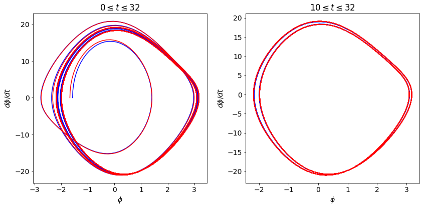
Let’s check the state space plots together:
fig_ss = plt.figure(figsize=(12,6))

ax_ss1 = fig_ss.add_subplot(1,2,1)
start, stop = start_stop_indices(t_pts, 0., 32)
plot_y_vs_x(phi_1[start : stop], phi_dot_1[start : stop],
            axis_labels=state_space_labels,
            color='blue',
            label=None,
            title=rf'$0 \leq t \leq 32$',
            ax=ax_ss1)
plot_y_vs_x(phi_2[start : stop], phi_dot_2[start : stop],
            axis_labels=state_space_labels,
            color='red',
            label=None,
            title=None,
            ax=ax_ss1)

# now skip the transients
ax_ss2 = fig_ss.add_subplot(1,2,2)
start, stop = start_stop_indices(t_pts, 10., 32)
plot_y_vs_x(phi_1[start : stop], phi_dot_1[start : stop],
            axis_labels=state_space_labels,
            color='blue',
            label=None,
            title=rf'$10 \leq t \leq 32$',
            ax=ax_ss2)
plot_y_vs_x(phi_2[start : stop], phi_dot_2[start : stop],
            axis_labels=state_space_labels,
            color='red',
            label=None,
            title=None,
            ax=ax_ss2)

fig_ss.tight_layout()
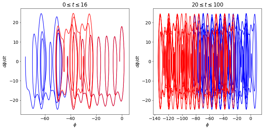
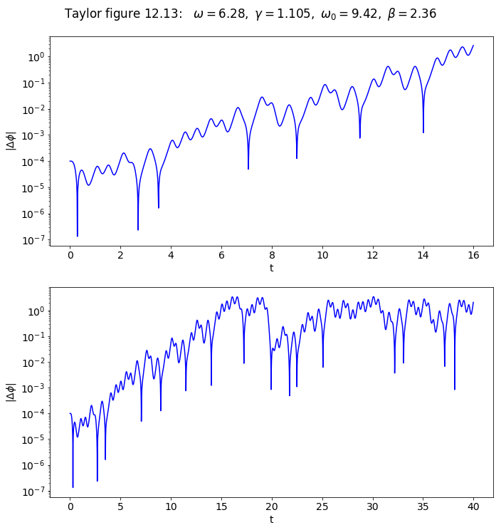
Make plots for Taylor figure 12.13: Looking at \(\Delta\phi\) for \(\gamma = 1.105\)#
# Labels for individual plot axes
phi_vs_time_labels = (r'$t$', r'$\phi(t)$')
Delta_phi_vs_time_labels = (r'$t$', r'$\Delta\phi(t)$')
phi_dot_vs_time_labels = (r'$t$', r'$d\phi/dt(t)$')
state_space_labels = (r'$\phi$', r'$d\phi/dt$')

# Common plotting time (generate the full time then use slices)
t_start = 0.
t_end = 100.
delta_t = 0.01

t_pts = np.arange(t_start, t_end+delta_t, delta_t)

# Common pendulum parameters
gamma_ext = 1.105
omega_ext = 2.*np.pi
phi_ext = 0.

omega_0 = 1.5*omega_ext
beta = omega_0/4.

# Instantiate a pendulum
p1 = Pendulum(omega_0=omega_0, beta=beta,
              gamma_ext=gamma_ext, omega_ext=omega_ext, phi_ext=phi_ext)

# calculate the driving force for t_pts
driving = p1.driving_force(t_pts)
Set abserr and relerr to 1.e-10 from the beginning.
# make a plot of Delta phi for same pendulum but two different initial conds
phi_0_1 = -np.pi / 2.
phi_dot_0 = 0.0
phi_1, phi_dot_1 = p1.solve_ode(phi_0_1, phi_dot_0,
                                abserr=1.e-10, relerr=1.e-10)

phi_0_2 = phi_0_1 + 1.e-4   # .1 radian lower
phi_dot_0 = 0.0
phi_2, phi_dot_2 = p1.solve_ode(phi_0_2, phi_dot_0,
                                abserr=1.e-10, relerr=1.e-10)

# Calculate the absolute value of \phi_2 - \phi_1
Delta_phi = np.fabs(phi_2 - phi_1)

# Change the common font size
font_size = 14
plt.rcParams.update({'font.size': font_size})

# start the plot!
fig = plt.figure(figsize=(10,10))
overall_title = 'Taylor figure 12.13:  ' + \
                rf' $\omega = {omega_ext:.2f},$' + \
                rf' $\gamma = {gamma_ext:.3f},$' + \
                rf' $\omega_0 = {omega_0:.2f},$' + \
                rf' $\beta = {beta:.2f}$' + \
                '\n'     # \n means a new line (adds some space here)
fig.suptitle(overall_title, va='baseline')

# two plot: plot from t=0 to t=8 and another from t=0 to t=16
ax_a = fig.add_subplot(2,1,1)

start, stop = start_stop_indices(t_pts, 0., 16.)
ax_a.semilogy(t_pts[start : stop], Delta_phi[start : stop],
            color='blue', label=None)
ax_a.set_xlabel('t')
ax_a.set_ylabel(r'$|\Delta\phi|$')

ax_b = fig.add_subplot(2,1,2)

start, stop = start_stop_indices(t_pts, 0., 40.)
plot_y_vs_x(t_pts[start : stop], Delta_phi[start : stop],
            color='blue', label=None, semilogy=True)
ax_b.set_xlabel('t')
ax_b.set_ylabel(r'$|\Delta\phi|$')

fig.tight_layout()
# always bbox_inches='tight' for best results.  Further adjustments also.
fig.savefig('figure_12.13.png', bbox_inches='tight')
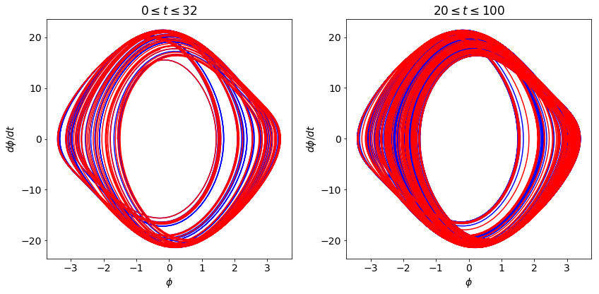
Let’s check the state space plots together:
fig_ss = plt.figure(figsize=(12,6))

ax_ss1 = fig_ss.add_subplot(1,2,1)
start, stop = start_stop_indices(t_pts, 0., 32)
plot_y_vs_x(phi_1[start : stop], phi_dot_1[start : stop],
            axis_labels=state_space_labels,
            color='blue',
            label=None,
            title=rf'$0 \leq t \leq 32$',
            ax=ax_ss1)
plot_y_vs_x(phi_2[start : stop], phi_dot_2[start : stop],
            axis_labels=state_space_labels,
            color='red',
            label=None,
            title=None,
            ax=ax_ss1)

# now skip the transients
ax_ss2 = fig_ss.add_subplot(1,2,2)
start, stop = start_stop_indices(t_pts, 20., 100)
plot_y_vs_x(phi_1[start : stop], phi_dot_1[start : stop],
            axis_labels=state_space_labels,
            color='blue',
            label=None,
            title=rf'$20 \leq t \leq 100$',
            ax=ax_ss2)
plot_y_vs_x(phi_2[start : stop], phi_dot_2[start : stop],
            axis_labels=state_space_labels,
            color='red',
            label=None,
            title=None,
            ax=ax_ss2)

fig_ss.tight_layout()
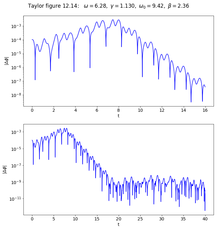
Make plots for Taylor figure 12.14: Looking at \(\Delta\phi\) for \(\gamma = 1.13\)#
# Labels for individual plot axes
phi_vs_time_labels = (r'$t$', r'$\phi(t)$')
Delta_phi_vs_time_labels = (r'$t$', r'$\Delta\phi(t)$')
phi_dot_vs_time_labels = (r'$t$', r'$d\phi/dt(t)$')
state_space_labels = (r'$\phi$', r'$d\phi/dt$')

# Common plotting time (generate the full time then use slices)
t_start = 0.
t_end = 100.
delta_t = 0.01

t_pts = np.arange(t_start, t_end+delta_t, delta_t)

# Common pendulum parameters
gamma_ext = 1.13
omega_ext = 2.*np.pi
phi_ext = 0.

omega_0 = 1.5*omega_ext
beta = omega_0/4.

# Instantiate a pendulum
p1 = Pendulum(omega_0=omega_0, beta=beta,
              gamma_ext=gamma_ext, omega_ext=omega_ext, phi_ext=phi_ext)

# calculate the driving force for t_pts
driving = p1.driving_force(t_pts)
Set abserr and relerr to 1.e-10 from the beginning.
# make a plot of Delta phi for same pendulum but two different initial conds
phi_0_1 = -np.pi / 2.
phi_dot_0 = 0.0
phi_1, phi_dot_1 = p1.solve_ode(phi_0_1, phi_dot_0,
                                abserr=1.e-10, relerr=1.e-10)

phi_0_2 = phi_0_1 + 1.e-4   # 10^{-3} radian lower
phi_dot_0 = 0.0
phi_2, phi_dot_2 = p1.solve_ode(phi_0_2, phi_dot_0,
                                abserr=1.e-10, relerr=1.e-10)

# Calculate the absolute value of \phi_2 - \phi_1
Delta_phi = np.fabs(phi_2 - phi_1)

# Change the common font size
font_size = 14
plt.rcParams.update({'font.size': font_size})

# start the plot!
fig = plt.figure(figsize=(10,10))
overall_title = 'Taylor figure 12.14:  ' + \
                rf' $\omega = {omega_ext:.2f},$' + \
                rf' $\gamma = {gamma_ext:.3f},$' + \
                rf' $\omega_0 = {omega_0:.2f},$' + \
                rf' $\beta = {beta:.2f}$' + \
                '\n'     # \n means a new line (adds some space here)
fig.suptitle(overall_title, va='baseline')

# two plot: plot from t=0 to t=8 and another from t=0 to t=16
ax_a = fig.add_subplot(2,1,1)

start, stop = start_stop_indices(t_pts, 0., 16.)
ax_a.semilogy(t_pts[start : stop], Delta_phi[start : stop],
            color='blue', label=None)
ax_a.set_xlabel('t')
ax_a.set_ylabel(r'$|\Delta\phi|$')

ax_b = fig.add_subplot(2,1,2)

start, stop = start_stop_indices(t_pts, 0., 40.)
plot_y_vs_x(t_pts[start : stop], Delta_phi[start : stop],
            color='blue', label=None, semilogy=True)
ax_b.set_xlabel('t')
ax_b.set_ylabel(r'$|\Delta\phi|$')

fig.tight_layout()
# always bbox_inches='tight' for best results.  Further adjustments also.
fig.savefig('figure_12.14.png', bbox_inches='tight')
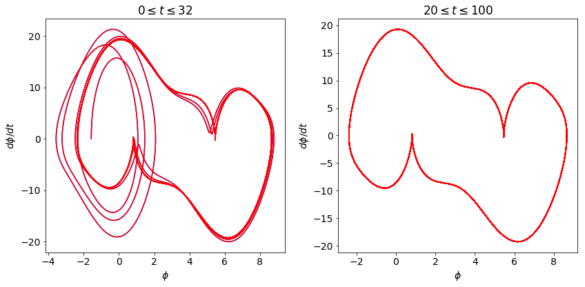
Let’s check the state space plots together:
fig_ss = plt.figure(figsize=(12,6))

ax_ss1 = fig_ss.add_subplot(1,2,1)
start, stop = start_stop_indices(t_pts, 0., 32)
plot_y_vs_x(phi_1[start : stop], phi_dot_1[start : stop],
            axis_labels=state_space_labels,
            color='blue',
            label=None,
            title=rf'$0 \leq t \leq 32$',
            ax=ax_ss1)
plot_y_vs_x(phi_2[start : stop], phi_dot_2[start : stop],
            axis_labels=state_space_labels,
            color='red',
            label=None,
            title=None,
            ax=ax_ss1)

# now skip the transients
ax_ss2 = fig_ss.add_subplot(1,2,2)
start, stop = start_stop_indices(t_pts, 20., 100)
plot_y_vs_x(phi_1[start : stop], phi_dot_1[start : stop],
            axis_labels=state_space_labels,
            color='blue',
            label=None,
            title=rf'$20 \leq t \leq 100$',
            ax=ax_ss2)
plot_y_vs_x(phi_2[start : stop], phi_dot_2[start : stop],
            axis_labels=state_space_labels,
            color='red',
            label=None,
            title=None,
            ax=ax_ss2)

fig_ss.tight_layout()
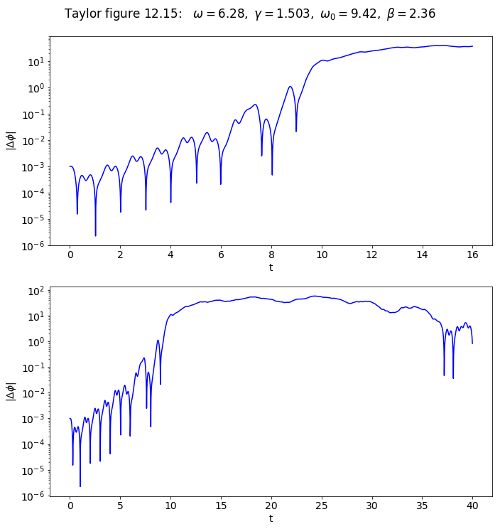
Make plots for Taylor figure 12.15: Looking at \(\Delta\phi\) for \(\gamma = 1.503\)#
# Labels for individual plot axes
phi_vs_time_labels = (r'$t$', r'$\phi(t)$')
Delta_phi_vs_time_labels = (r'$t$', r'$\Delta\phi(t)$')
phi_dot_vs_time_labels = (r'$t$', r'$d\phi/dt(t)$')
state_space_labels = (r'$\phi$', r'$d\phi/dt$')

# Common plotting time (generate the full time then use slices)
t_start = 0.
t_end = 100.
delta_t = 0.01

t_pts = np.arange(t_start, t_end+delta_t, delta_t)

# Common pendulum parameters
gamma_ext = 1.503
omega_ext = 2.*np.pi
phi_ext = 0.

omega_0 = 1.5*omega_ext
beta = omega_0/4.

# Instantiate a pendulum
p1 = Pendulum(omega_0=omega_0, beta=beta,
              gamma_ext=gamma_ext, omega_ext=omega_ext, phi_ext=phi_ext)

# calculate the driving force for t_pts
driving = p1.driving_force(t_pts)
Set abserr and relerr to 1.e-10 from the beginning.
# make a plot of Delta phi for same pendulum but two different initial conds
phi_0_1 = -np.pi / 2.
phi_dot_0 = 0.0
phi_1, phi_dot_1 = p1.solve_ode(phi_0_1, phi_dot_0,
                                abserr=1.e-10, relerr=1.e-10)

phi_0_2 = phi_0_1 + 1.e-3   # 10^{-3} radian lower
phi_dot_0 = 0.0
phi_2, phi_dot_2 = p1.solve_ode(phi_0_2, phi_dot_0,
                                abserr=1.e-10, relerr=1.e-10)

# Calculate the absolute value of \phi_2 - \phi_1
Delta_phi = np.fabs(phi_2 - phi_1)

# Change the common font size
font_size = 14
plt.rcParams.update({'font.size': font_size})

# start the plot!
fig = plt.figure(figsize=(10,10))
overall_title = 'Taylor figure 12.15:  ' + \
                rf' $\omega = {omega_ext:.2f},$' + \
                rf' $\gamma = {gamma_ext:.3f},$' + \
                rf' $\omega_0 = {omega_0:.2f},$' + \
                rf' $\beta = {beta:.2f}$' + \
                '\n'     # \n means a new line (adds some space here)
fig.suptitle(overall_title, va='baseline')

# two plot: plot from t=0 to t=8 and another from t=0 to t=16
ax_a = fig.add_subplot(2,1,1)

start, stop = start_stop_indices(t_pts, 0., 16.)
ax_a.semilogy(t_pts[start : stop], Delta_phi[start : stop],
            color='blue', label=None)
ax_a.set_xlabel('t')
ax_a.set_ylabel(r'$|\Delta\phi|$')

ax_b = fig.add_subplot(2,1,2)

start, stop = start_stop_indices(t_pts, 0., 40.)
plot_y_vs_x(t_pts[start : stop], Delta_phi[start : stop],
            color='blue', label=None, semilogy=True)
ax_b.set_xlabel('t')
ax_b.set_ylabel(r'$|\Delta\phi|$')

fig.tight_layout()
# always bbox_inches='tight' for best results.  Further adjustments also.
fig.savefig('figure_12.15.png', bbox_inches='tight')
# Change the common font size
font_size = 14
plt.rcParams.update({'font.size': font_size})
# start the plot!
fig = plt.figure(figsize=(10,10))
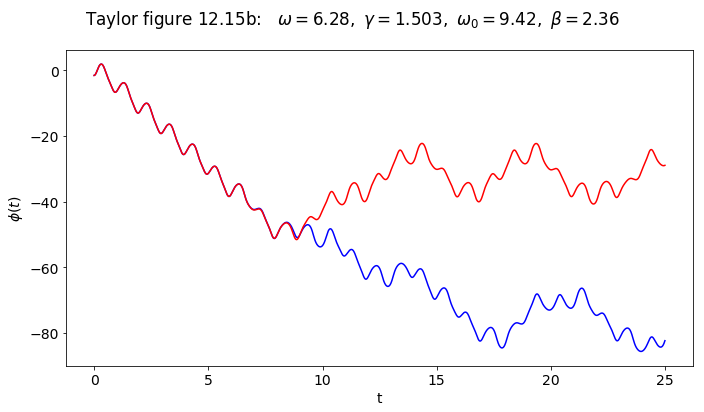
overall_title = 'Taylor figure 12.15b: ' + \
rf' $\omega = {omega_ext:.2f},$' + \
rf' $\gamma = {gamma_ext:.3f},$' + \
rf' $\omega_0 = {omega_0:.2f},$' + \
rf' $\beta = {beta:.2f}$' + \
'\n' # \n means a new line (adds some space here)
fig.suptitle(overall_title, va='baseline')
# two plot: plot from t=0 to t=8 and another from t=0 to t=25
ax_a = fig.add_subplot(2,1,1)
start, stop = start_stop_indices(t_pts, 0., 25.)
ax_a.plot(t_pts[start : stop], phi_1[start : stop],
color='blue', label=None)
ax_a.plot(t_pts[start : stop], phi_2[start : stop],
color='red', label=None)
ax_a.set_xlabel('t')
ax_a.set_ylabel(r'$\phi(t)$')
fig.tight_layout()
# always bbox_inches='tight' for best results. Further adjustments also.
#fig.savefig('figure_12.15b.png', bbox_inches='tight')
Let’s check the state space plots together:
fig_ss = plt.figure(figsize=(12,6))

ax_ss1 = fig_ss.add_subplot(1,2,1)
start, stop = start_stop_indices(t_pts, 0., 16)
plot_y_vs_x(phi_1[start : stop], phi_dot_1[start : stop],
            axis_labels=state_space_labels,
            color='blue',
            label=None,
            title=rf'$0 \leq t \leq 16$',
            ax=ax_ss1)
plot_y_vs_x(phi_2[start : stop], phi_dot_2[start : stop],
            axis_labels=state_space_labels,
            color='red',
            label=None,
            title=None,
            ax=ax_ss1)

# now skip the transients
ax_ss2 = fig_ss.add_subplot(1,2,2)
start, stop = start_stop_indices(t_pts, 20., 100)
plot_y_vs_x(phi_1[start : stop], phi_dot_1[start : stop],
            axis_labels=state_space_labels,
            color='blue',
            label=None,
            title=rf'$20 \leq t \leq 100$',
            ax=ax_ss2)
plot_y_vs_x(phi_2[start : stop], phi_dot_2[start : stop],
            axis_labels=state_space_labels,
            color='red',
            label=None,
            title=None,
            ax=ax_ss2)

fig_ss.tight_layout()