Yet another way to solve the Schrodinger equation

We have seen how to solve the Schrodinger equation for bound state energies and wave functions using a matrix representation in coordinate space, a matrix representation in a harmonic oscillator basis, and using path integrals. In this notebook we add another method to the list: direct solution of the S-equation in coordinate space as a differential equation using finite difference methods.

Solving as a differential equation in coordinate representation.

This works when we have a local potential (otherwise the Schrodinger equation is an integro-differential equation in coordinate representation). If we have a central potential in three dimensions, the potential depends only on \(r\):

\[ V({\bf x}) = V(|{\bf x}|) \equiv V(r) \ , \]

and we can use a partial wave decomposition (which means we separate the equation in spherical coordinates). That is, we write

\[ \Psi_{nlm}({\bf x}) = \frac{u_{nl}(r)}{r} Y_{lm}(\theta,\phi) \ , \]

where \(Y_{lm}\) is a spherical harmonic, and solve the radial one-dimensional Schrodinger equation:

\[ -\frac{\hbar^2}{2M}\frac{d^2u_{nl}(r)}{dr^2} + \underbrace{\biggl[ V(r) + \frac{\hbar^2 l (l+1)}{2M r^2} \biggr]}_{\equiv V_{\rm eff}(r)} u_{nl}(r) = E_n u_{nl}(r) \ , \label{eq:radSE} \]

with

\[ u_{nl}(r=0) = 0 \qquad \mbox{and} \qquad \int_0^\infty |u_{nl}(r)|^2\, dr = 1 \ . \label{eq:radbc} \]

We’ll apply this method here for radial equations with a central potential.

For the Coulomb potential \(V(r)= -Ze^2/r\), we use the notation \(N\) instead of \(n\) for the number of nodes and define

\[ n = N + \ell + 1, \]

because the energies will only depend on \(n\) (more precisely, on \(1/n^2\)).

Solving the differential equation using a finite difference method

Here we use a (crude) finite difference formula for the second derivative in the kinetic energy operator (here with notation appropriate to the radial equation in spherical coordinates and \(h \equiv \Delta x\)):

\[ \frac{d^2u}{dr^2} = \frac{u(r+h) - 2 u(r) + u(r-h)}{h^2} + {\cal O}(h^2) . \]

You can verify this approximation by expanding \(u(r+h)\) and \(u(r-h)\) in Taylor series about \(u(r)\). We’ll label the points:

\[ r_i = i\times h\ , \qquad i = 0,1,2,\cdots,N-1 \]

where \(N\) is the number of steps and the step size \(h\) is given by:

\[ h = \frac{R_{\rm max}}{N-1} . \]

Thus, \(r_0 = 0\), \(r_1 = h\), and so on up to \(r_{N} = (N-1)h = R_{\rm max}\).

We can rearrange the equation to let us determine the radial wave function \(u(r)\) at successive steps in \(h\), given the previous two values of \(u\):

(1)\[\begin{align} u(r+h) &= 2 u(r) - u(r-h) + h^2\frac{d^2u}{dr^2} \\ &= 2 u(r) - u(r-h) + h^2\left[\frac{2m}{\hbar^2}(V_{\rm eff}(r)-E) \right]u(r) \end{align}\]

For \(h>0\) we integrate out from the origin, starting with two initial values, while for \(h < 0\) we integrate in from a sufficiently large value of \(r\) (our approximation to \(\infty\)), where “sufficiently large” means that we are in the asymptotic region.

import numpy as np
from scipy.integrate import quad, simps, solve_ivp

import matplotlib.pyplot as plt
import seaborn as sns; sns.set_style("darkgrid"); sns.set_context("talk")

1. Set Hamiltonian constants, nodes and \(\ell\), and mesh/iteration parameters

If we set the important quantities \(\hbar\), \(m\), and \(Ze^2\) all equal to one (i.e., we measure in units where these are one), then the exact energy eigenvalues are

\[ E_n = -\frac{1}{2n^2}. \]

# values of constants (choose natural units)
hbar = 1;
mass = 1;  
Ze_sq = 1;   # Z factor (Z = 1 for hydrogen) times electron charge squared

Here is where you set the desired number of nodes and the value of \(\ell\). You might also want to change the initial guess of E_trial for some choices of nodes and \(\ell\).

nodes = 0  # desired number of nodes in radial wave function
ell = 0    # orbital angular momentum quantum number
E_trial = -0.1      # initial guess for the trial wf
DeltaE_nodes = .02  # small increment in energy if no. of nodes is incorrect
iter_max = 40  # maximum number of iterations

Here is where you can adjust the properties of the radial mesh, such as the number of points, the maximum \(r\) value (which together sets \(h \equiv \Delta r\)). Particularly important is that you set the matching index i_match, which you will have to adjust when you change the number of nodes and the value of \(\ell\).

N_pts = 2001   # For accuracy this should be large; over 1000 
r_min = 0.     # For three-dimensions, r starts at zero
r_max = 20.    # How large to make this depends on the potential
Delta_r = (r_max - r_min) / (N_pts - 1)
r_mesh = np.linspace(r_min, r_max, N_pts)  # create the grid ("mesh") of x points
i_match = int(N_pts / 4)   # where to match in and out solutions (adjust as needed)

C_out = 1.  # coefficient for approximate analytic solution near origin
D_in = 1.e-40  # coefficient for approximate analytic solution at large r
DeltaE_tol = 0.0001  # stop iterating when DeltaE_trial < DeltaE_tol

u_out = np.zeros(N_pts)   # initialize array for radial wf from outward integration
u_in = np.zeros(N_pts)    # initialize array for radial wf from inwar integration
u_trial = np.zeros(N_pts) # initial array for scaled and joined radial wf 

2. Main iteration

Keep going until DeltaE_trial is less than (or equal to) DeltaE_tol.

# Evaluate the Coulomb potential on the mesh
V_on_mesh = -Ze_sq / r_mesh[1:] + hbar**2 / (2*mass) * ell * (ell + 1) / r_mesh[1:]**2
u_out[0] = 0

DeltaE_trial = 2 * DeltaE_tol  # initialize DeltaE_trial so there is at least one iteration
iter_num = 0
while np.abs(DeltaE_trial) > DeltaE_tol:
    # initialize the node count and increment the iteration number
    node_count = 0
    iter_num = iter_num + 1
    if iter_num > iter_max:
        print(f' *** Stopped at {iter_num} iterations ***')
        break

    # Set up the array for d^2u/dr^2 
    T_array = 2 * mass / hbar**2 * (V_on_mesh - E_trial)
     
    # integrate out from the origin, with analytic starting points
    u_out[1] = C_out * r_mesh[1]**(ell + 1)
    u_out[2] = C_out * r_mesh[2]**(ell + 1)
    
    for i in np.arange(1, i_match+2):
        u_out[i+1] = 2*u_out[i] - u_out[i-1] + Delta_r**2 * T_array[i] * u_out[i]
        # check for node
        if u_out[i+1] * u_out[i] < 0:
            node_count = node_count + 1
       
    # integrate in from the largest mesh point, using the asymptotic for of u(r)
    kappa = np.sqrt(-2*mass*E_trial / hbar**2)
    u_in[N_pts-1] = D_in * np.exp(-kappa * r_mesh[N_pts-1])
    u_in[N_pts-2] = D_in * np.exp(-kappa * r_mesh[N_pts-2])
    
    for i in np.arange(N_pts-2, i_match-2, -1, dtype=int):
        u_in[i-1] = 2*u_in[i] - u_in[i+1] + Delta_r**2 * T_array[i] * u_in[i]
        # check for node
        if u_in[i-1] * u_in[i] < 0:
            node_count = node_count + 1

    rescale = u_out[i_match] / u_in[i_match]
    u_in = rescale * u_in
        
    # join the out and in solutions at i_match
    u_trial = np.append(u_out[0:i_match], u_in[i_match:])
    
    # normalize the joined and scaled trial wave function u_trial
    u_trial = u_trial / np.sqrt(simps(u_trial**2, r_mesh))
    # print(f'norm check {simps(u_trial**2, r_mesh)}')   # debugging check
    
            
    # adjust trial energy, first by checking if node_count = nodes and then using formula
    if (node_count < nodes):  # too few nodes, increase trial energy by constant
        E_trial = E_trial + DeltaE_nodes
    elif (node_count > nodes):  # too many nodes, decrease trial energy by constant
        E_trial = E_trial - DeltaE_nodes

    else:  # correct no. of nodes; use formula to adjust trial energy         
        u_deriv_out = (u_out[i_match+1] - u_out[i_match-1]) / (2 * Delta_r)
        u_deriv_in = (u_in[i_match+1] - u_in[i_match-1]) / (2 * Delta_r)
        # print(f'u_deriv_out: {u_deriv_out},  u_deriv_in: {u_deriv_in}') # debugging
        
        norm = simps(u_trial**2, r_mesh)  # Should be equal to one
        DeltaE_trial =  -u_trial[i_match] * (u_deriv_in - u_deriv_out) / norm
        new_E_trial = E_trial + DeltaE_trial # New estimate for E_trial
        if new_E_trial > 0:
            E_trial = E_trial + 0.05 * DeltaE_trial
        else:
            E_trial = new_E_trial  
        
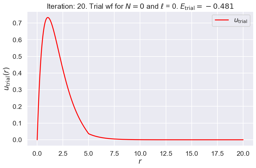
        # make a plot of the wave function
        fig = plt.figure(figsize=(10,6))
        
        ax1 = fig.add_subplot(1,1,1)
        ax1.set_xlabel(r'$r$')
        ax1.set_ylabel(r'$u_{\rm trial}(r)$')
        
        #ax1.set_xlim(0, r_max)
        #ax1.set_ylim(-1., 3)
        
        ax1.plot(r_mesh, u_trial, color='red', label=r'$u_{\rm trial}$')
         
        title_string = fr'Iteration: {iter_num}. ' \
                        + fr'Trial wf for $N = {nodes}$ and $\ell$ = {ell}.' \
                        + fr' $E_{{\rm trial}} = {E_trial:.3f}$'
        ax1.set_title(title_string)
        
        ax1.legend();
        

    # print current status
    print(f'\n**** Iteration #{iter_num}' )
    print(f'nodes: {node_count}, E_trial: {E_trial:.4f}, Delta E_trial: {DeltaE_trial:.5f}' )

**** Iteration #1
nodes: 1, E_trial: -0.1200, Delta E_trial: 0.00020

**** Iteration #2
nodes: 1, E_trial: -0.1400, Delta E_trial: 0.00020

**** Iteration #3
nodes: 1, E_trial: -0.1600, Delta E_trial: 0.00020

**** Iteration #4
nodes: 1, E_trial: -0.1800, Delta E_trial: 0.00020

**** Iteration #5
nodes: 1, E_trial: -0.2000, Delta E_trial: 0.00020

**** Iteration #6
nodes: 1, E_trial: -0.2200, Delta E_trial: 0.00020

**** Iteration #7
nodes: 1, E_trial: -0.2400, Delta E_trial: 0.00020

**** Iteration #8
nodes: 1, E_trial: -0.2600, Delta E_trial: 0.00020

**** Iteration #9
nodes: 1, E_trial: -0.2800, Delta E_trial: 0.00020

**** Iteration #10
nodes: 1, E_trial: -0.3000, Delta E_trial: 0.00020

**** Iteration #11
nodes: 1, E_trial: -0.3200, Delta E_trial: 0.00020

**** Iteration #12
nodes: 1, E_trial: -0.3400, Delta E_trial: 0.00020

**** Iteration #13
nodes: 1, E_trial: -0.3600, Delta E_trial: 0.00020

**** Iteration #14
nodes: 1, E_trial: -0.3800, Delta E_trial: 0.00020

**** Iteration #15
nodes: 1, E_trial: -0.4000, Delta E_trial: 0.00020

**** Iteration #16
nodes: 1, E_trial: -0.4200, Delta E_trial: 0.00020

**** Iteration #17
nodes: 1, E_trial: -0.4400, Delta E_trial: 0.00020

**** Iteration #18
nodes: 1, E_trial: -0.4600, Delta E_trial: 0.00020

**** Iteration #19
nodes: 1, E_trial: -0.4800, Delta E_trial: 0.00020

**** Iteration #20
nodes: 0, E_trial: -0.4811, Delta E_trial: -0.00114

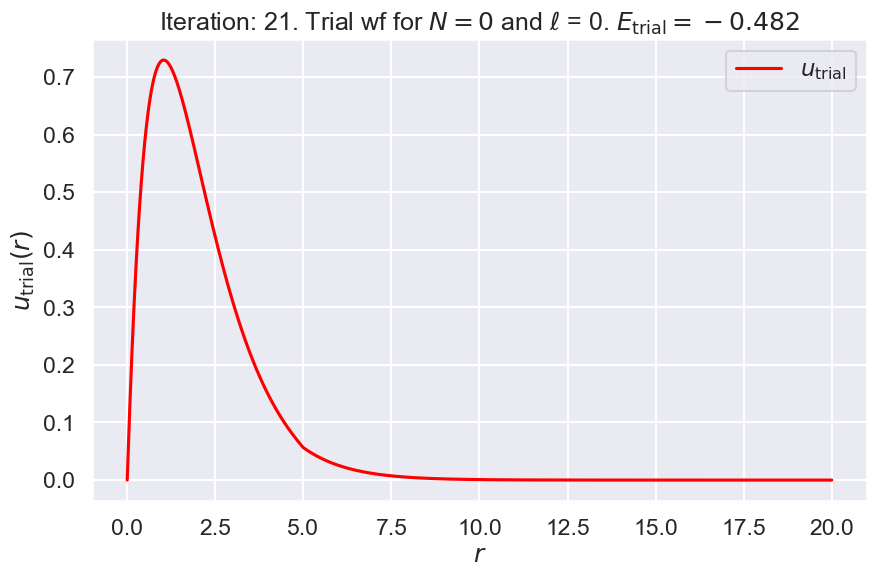
**** Iteration #21
nodes: 0, E_trial: -0.4820, Delta E_trial: -0.00083

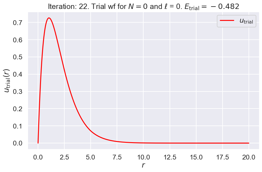
**** Iteration #22
nodes: 0, E_trial: -0.4821, Delta E_trial: -0.00016

**** Iteration #23
nodes: 0, E_trial: -0.4821, Delta E_trial: 0.00001

3. Output final result

# Final result
print(f'\n\n *** Calculated energy for {nodes} nodes and angular momentum {ell} is {E_trial:.4f}.' )

 *** Calculated energy for 0 nodes and angular momentum 0 is -0.4821.